5. Bayesian Modelling#
5.1. Bayesian probability#
The greek philosopher Aristotle formally introduced the field of Logic as the tool of deduction and therefore one of the the main tools of scientific progress. Logic allows to derive conclusions based on propositions that are taken for granted. Those propositions might have been themselves derived in a logical way, or might be principles that cannot be derived themselves, the starting building blocks of any theory or discipline.
A fundamental principle of logic is that of the “excluded third”, for which a given proposition can only be either true or false, but there is not a third option. Therefore, logic is based on the assumption of complete certainty about the propositions, both the premises and the conclusions. But most of our knowledge (if not all, as defended by empiricists like David Hume) is uncertain, therefore we need a tool that allows us to derive conclusions from uncertain premises. Under the so-called Bayesian school of probability, such a tool is probability theory, whose rules, that where inferred for the analysis of more specific toy cases like games of chance, we will see that turn out to apply to the wider case of reasoning under uncertainty.
In the Bayesian interpretation, a probability is a statement or our degree of belief in a proposition. For instance, the proposition “Apple stock will close tomorrow at a higher price than today” is, from today’s point of view, neither true or false. The application of logic is limited to situations where we have already observed the price of Apple tomorrow, and therefore we know if the proposition is true or false. However, we might be interested in making decisions today based on our confidence in the proposition without having to wait to know its trueness: we might trigger different trading strategies whose profits are linked to Apple stock depending on the degree of confidence on the proposition. Such way of reasoning happens in all spheres of our lives, where we are always looking ahead to un uncertain future: from minor decisions like which clothes to wear on a given day, to major ones like which professional career to follow.
What probability theory offers is a tool to be able to derive consistently degrees of belief on certain outcomes based on the degrees of belief on the premises. In our previous example, with probability theory we could potentially compute the probability of profit from a certain trading strategy based on the probability of Apple trading higher tomorrow. Our brains are capable of doing such calculations intuitively in familiar situations, but such intuition breaks down quickly in unfamiliar domains, when probabilities are very small, or when there is a large number of assumptions or outcomes. Probability as an extension of logic can compute these probabilities in any situation.
As we mentioned above, the actual rules to operate consistently with probabilities were inferred initially in the analysis of specific problems like games of chance or combinatorial problems, as done by mathematicians like Bernoulli and de Moivre in the 18th century. In the same century, reverend Thomas Bayes would write about application of probability theory to more general problems of reasoning under uncertainty, hence the name Bayesian school. It is important, however, to remark that Bayes was not the first author to attach such interpretation to probability, nor the one that would really formalize it as a proper theory of inference. That would be really Laplace, who successfully showed how to use the rules of probability to assign probabilities to propositions of interest to the scientific domain, the most famous probably being his work inferring the mass of Saturn from noisy observations.
That we can operate with the rules of probability theory to work on degrees of belief was not, however, properly analyzed until the work of the physicist Richard Cox in the 20th century. In his work from 1946, he starts from the basic idea of quantifying our degree of belief in a proposition by associating a real number to it, without necessarily linking it to probabilities. The only condition is that the larger the number, the larger must be our degree of belief. Then, he moves onto imposing consistency rules using logical reasoning:
If we specify how much we believe a proposition X is true, we are implicitly specifying how much we believe it is false
If we specify how much we believe a proposition Y is true, and then how much another proposition X is true, given that Y is true, then we are implicitly specifying how much we believe both X and Y to be true
Then, using Boolean logic and ordinary algebra, he found that consistency constraints this real numbers associated to our degree of belief to follow the rules of probability theory:
where ̄X denotes the proposition that X is false. Therefore, if we are bound to use the rules of logical reasoning, we can see that our degrees of belief can be rigorously mapped to probability theory.
These rules are just the basic building blocks from probability theory. Many other results can be derived from them, for instance the infamous Bayes’ theorem, which is a simple consequence of the product rule. Since we can write the product rule either way in terms of X or Y:
Then:
which is Bayes’s theorem. We also could derive the marginalization rule:
by taking the continuum limit starting from a discrete and complete set of events. We leave it as an exercise for the interested reader.
The work of Cox was continued by E.T. Jaynes, who would extensively work on the interpretation of probability as an extension of deductive logic, and tackle many of the controversial views on this interpretation –like the role of prior probabilities that we will discuss later on. Another typical criticism is its supposedly lack of objectivity as a universal theory of knowledge, since degrees of belief are attached to individuals and therefore they lack the objectivity needed for consensual agreement on the validity of a proposition. As Jaynes points out, such subjectivity disappears if we introduce explicitly the set of information available to the observers: two rational observers with the same information available must agree on the degrees of belief assigned to a proposition, otherwise either they are not rational or they don’t share the same information. We can formalize this by introducing the set of information available, \(I\) into the definition of the probabilities, namely \(P(X|I)\).
5.1.1. Probability as an extension of logic#
So far we have seen how we can map the rules of consistent reasoning based on degrees of belief to probability theory. Let us now go back to the link to deductive logic. A basic syllogism in logic is
So if \(A\) is true, then \(B\) is true. Let us discuss a few ways this syllogism is affected by uncertain.
A first situation happens when the proposition \(A \implies B\) itself is true, but we only have a degree of belief on \(A\), expressed by probability \(P(A)\). If we are interested in the degree of belief on \(B\), We can use the marginalization rule to write \(P(B) = P(B|A) P(A) + P(B|\bar{A})P(\bar{A})\). Since the proposition \(A \implies B\) is translated into \(P(B|A) = 1\), hence \(P(B) = P(A) + P(B|\bar{A})P(\bar{A}) = P(A)(1- P(B|\bar{A})) + P(B|\bar{A})\). As expected, if \(P(A) = 1\) then \(P(B) = 1\), in agreement with deductive logic. However, when \(P(A) < 1\) the degree of belief on \(B\) depends on the other potential mechanisms that can trigger \(B\) when \(A\) is false, quantified by \(P(B|\bar{A})\)
A second situation is when proposition \(A \implies B\) is true, but we observe \(B\) and not \(A\). In this case we can use Bayes theorem:
Again, since \(P(B|A) = 1\), this simplifies to:
In this case, the probability of \(A\) contingent to the observation of \(B\) depends, as in the previous case, on the other ways that B can be triggered when \(A\) is false, but also on the so-called prior probability of A, \(P(A)\), i.e. the degree of belief on A that we had before observing B. In the same language, \(P(A|B)\) is called a posterior probability. A key consequence of this result is that \(P(A|B) > P(A)\), since \(P(B|\bar{A}) < 1\) (otherwise we could not have P(B|A) = 1), and therefore the denominator \(P(A) + P(B|\bar{A})P(\bar{A}) < P(A) + P(\bar{A}) = 1\). Despite the uncertainty, knowledge of \(B\) always increases our degree of belief on \(A\), i.e. we can derive useful knowledge out of the domain of deductive logic.
Prior and posterior probabilities play a key role in Bayesian probability theory. Bayes theorem allows us to consistently update our prior degrees of belief (probabilities) based on new observations, in the form of posterior degrees of belief. As it happens with premises in deductive logic, prior probabilities can themselves be the result of previous inferences, although at some point they might need to be provided based on different considerations than previous observations, that might not be recorded systematically. Since they are inherent to Bayesian reasoning, critics of this theory have pointed them out as a weakness, an artificial requirement that biases the conclusions that other theories could just infer from the available observations.
In reality, those alternative theories are the ones that make hidden assumptions that effectively set the prior probabilities to naive choices in an uncontrolled way. Bayesian probability is only mathematically stating the obvious: our degree of belief on a proposition is not only driven by a given set of observations, there is always potentially prior information that can be used to improve our estimations. And in the rare case when it is not, there are also ways to assign consistently prior probabilities, as we will see in the next section.
5.1.2. Assigning prior probabilities#
Theoretically, every prior probability could be written as a posterior probability conditional to previously observed data. This chain of probabilities can be exhausted in two ways: 1) because we don’t have on record any relevant data from which to compute posterior probabilities, 2) because such data does not exist, i.e. the proposition under analysis is completely agnostic to any data previously observed. Of course the latter makes for a deep philosophical discussion, which could be easily carried out to the beginning of the observed universe. In all practical terms, is case 1) the one we are faced with.
When there is not relevant data recorded to compute posterior probabilities that serve as priors for later computations, we need to find a different way to assign prior probabilities. The general idea is to exploit known properties or constraints of the problem analyzed.
A popular idea is assigning priori probabilities based on symmetries of the problem. In particular, we can use De Moivre’s computation of probability as a ratio of possible outcomes where a certain proposition is true:
This definition is suitable for situations like dice games where 1) the outcomes are countable, 2) there is a symmetry in each outcome, in the sense that they can be considered equiprobable.
A more general principle is that of maximum entropy, which generalizes the Moivre’s rule to more complicated propositions where our prior knowledge is based on limitations or constraints on the valid outcomes. Let us consider for simplicity a discrete set of outcomes \(i = 1, ..., N\) (which are themselves an exhaustive set of exclusive propositions), each with an a priori probability \(p_i\) that we want to determine. The entropy of this probability distribution is given, using Shanon’s definition, by:
The motivation for the entropy function is that it can be seen as arguably the most simple functional form that consistently quantifies the uncertainty of a probability distribution, versus other potential assignments like \(\sum_i p_i^2\) for instance that can be seen to run into inconsistencies.
If we admit not having more information about a specific problem apart from the possible outcomes, we can assign as prior probabilities those that maximize entropy, conditional of course to be a complete set of probabilities, i.e. they sum up to 1. We include this restriction by using a Lagrange multiplier, so our objective function reads:
We can know maximize this Lagrangian with respect to each \(p_i\), although out of symmetry we can see that any permutation \(i \rightarrow j\) leaves the functional invariant, so the solution must be \(p_1 = ... = p_N\) and using the constraint this means \(p_i = 1/N\) which recovers De Moivre’s rule.
More interesting are cases where we have extra restrictions. For instance, let us assume that our prior knowledge includes a restriction on the average of a random variable that takes values \(x_1, ..., x_N\) under each outcome, so we know:
Our constraint maximization problem now reads:
Notice that the symmetry argument does no longer hold, so we take derivatives to find the extreme:
The solution is
where \(Z\) is a normalization constant, usually called the partition function in Statistical Physics applications. This is an exponential or Gibbs distribution for the random variable \(x\). The Lagrange multiplier \(\lambda_2\) is related to the average \(\bar{X}\) by means of the constraint:
This also points out to a general property of the partition function in which the moments of the distribution can be computed by taking derivatives of the partition function with respect of \(\lambda_2\). It is usual to rewrite this term as \(\lambda_2 = 1 / T\), with T called the temperature in analogy to Statistical Physics.
Let us consider a final case in which we add a second restriction on the second momentum of the distribution of the random variable \(x\), namely \(\sum_i p_i x_i^2 = \bar{X_i^2}\). The restricted optimization target now reads:
Computation of the extreme yields:
The solution can be written as:
which properly normalized can be quickly recognized as a Gaussian distribution. As pointed out by Jaynes, that the Gaussian distribution is the maximum entropy distribution for a problem in which we know the mean and variance (via its second order momentum), can be seen as a motivation for its pervasiveness in all sorts of domains. It is a natural prior distribution for problems where we have knowledge of the scale of likely values of the phenomenon under observation.
To close this discussion, let us touch upon the question of non-informative priors, which seek to describe a situation in which there is not relevant knowledge a prior about the problem. It turns out this is not a simple topic, and such situation needs to be described with more precision. At the very least, we need to specify what we are ignorant about. Take the example of a parameter we are uncertain about, and we parametrize our belief about this parameter using a distribution with the form: \(f(\nu, \sigma)\), where \(\nu\) is a location parameter and \(\sigma\) is a scale parameter. This setup encompasses multiple real cases where we express our knowledge in terms of a most likely range of values. For instance, if \(f\) corresponds to a normal distribution, the range given by \(\nu \pm \sigma\) has a probability of approximately 68% of containing the true value of the parameter, according to our beliefs. What does it mean to have a non-informative prior in this case? Since we are already introducing some prior information in the structure of the problem, we can not really say that we are fully ignorant, so we need to be more precise.
A useful way to express such ignorance with precision is by using transformation groups and invariants of the problem. In this example, we could argue that having knowledge about the scale \(\sigma\) means that our prior \(f(\nu, \sigma)\) changes under a transformation of scale: \(\sigma \rightarrow a \sigma\). As commented by Jaynes (page 379), if a scale transformation makes the problem appear different to us, then we must have some prior information about the absolute scale. The same argument can be applied to the location \(\nu\): if a change of location \(\nu \rightarrow \nu + b\) affects our view of the problem, then we must have some prior information about the location of the parameter. If we change variables in a distribution it must hold:
In our case, since \(\nu' = \nu + b\) and \(\sigma' = a \sigma\), computing the Jacobian:
Now we can express the conditions for a non-informative prior by stating that such change of variables shall not make any difference to our prior distribution, since otherwise we would have indeed some knowledge about the scale or location of the problem. This means:
Therefore:
This equation must hold for any \(a\) and \(b\). Let us take \(a = 1\), in this case \(f(\nu + b, \sigma) = f(\nu, \sigma)\) which means that the function cannot depend on \(\nu\), hence \(f(\nu, \sigma) = \phi(\sigma)\). The resulting equation for a general \(a\) is \(\phi(a \sigma) = a^{-1} \phi(\sigma)\) whose general solution is \(\phi(\sigma) = \text{const} \,\sigma\). Therefore, the non-informative prior for this problem is:
which corresponds to the so-called Jeffrey’s non-informative prior for this particular problem. As mentioned, this prior is relevant for instance in the particular but very common case when we model our beliefs using a Gaussian distribution. Ignorance about the location or scale of the distribution of this parameter can only be consistently encoded by using the Jeffrey’s prior.
5.1.3. Bayesian inference and hypothesis testing#
Bayes’ theorem can be used as the main tool to guide a theory of rational inference under uncertainty, providing us with a way to quantify the quality of a hypothesis \(H\) about the world based on the evidence (observations) available \(E\)::
\(P(H|E) = \frac{P(E|H)}{P(E)} P(H)\)
A high score is achieved in different ways:
When the prior probability of the hypothesis is high, meaning that the hypothesis was belief to be true even before analyzing the evidence.
When the ratio \(\frac{P(E|H)}{P(E)}\) is high, meaning that the probability of the evidence under the hypothesis is higher than the probability in general of the evidence. This means that evidence that is generally thought to be unlikely (meaning that \(P(E)\) was small), when explained by the hypothesis (i.e. \(P(E|H)\) is now high), provides a stronger score to the hypothesis than those cases in which the evidence was generally probable in any case (\(P(E)\) is high). Of course the reverse is also true: when a theory fails to explain evidence that is generally considered likely, then the score for this hypothesis will be lower.
One strength of Bayesian hypothesis testing that correctly captures many attributes attached to the way scientific research is normally conducted:
Scientists seek to test hypothesis by deriving predictions that are relatively unlikely. For the most precise case of a deterministic prediction, this means that \(P(E|H) = 1\), and \(P(E)\) is small. This way, the ratio \(P(E|H) / P(E)\) is large, providing a strong support to the hypothesis in case the prediction is verified empirically.
Scientists that disagree on the validity of a hypothesis will score different prior probabilities to \(H\). However, if predictions that are strongly attributed to this hypothesis (and weekly to alternative ones) are confirmed, their posterior probabilities will tend to converge since the scientist that attached a lower prior probability for \(H\) will also attach naturally a lower probability to the prediction overall, \(P(E)\), by virtue of Bayes’ theorem:
\[P(E) = P(E|H)P(H) + P(E|\bar{H})P(\bar{H}) = P(H) + P(E|\bar{H})P(\bar{H})\]This scientist therefore will need to update her posterior probability by a factor \(1/P(E)\) larger than the one that originally believed in the truth of the hypothesis, since, assuming that \(P(E|\bar{H}) < 1\), then:
\[P(H) + P(E|\bar{H})P(\bar{H}) = P(H)(1-P(E|\bar{H})) + P(E|\bar{H})\]and hence \(P(E)\) is smaller for the scientist who attributes a lower prior probability to \(P(H)\). This implies a larger update of the posterior relative to the prior for the skeptic scientist, which implies a convergence in posteriors with the other scientist.
Scientists score higher hypotheses whose predictions have been validated multiple times independently, but the marginal increase in the score tends to decrease with the number of repetitions. In terms of Bayes’ theorem, this is reflected in the fact that as a prediction is validated thanks to evidences \(E_i\) in agreement with the prediction, \(P(E_1) < P(E_2) < P(E_3) <...\), and given the upper bound \(P(E) \leq 1\), the convergence rate necessarily decreases when enough evidence is accumulated. The mechanics is the same as in the previous argument regarding scientists with different priors for a given hypothesis.
Finally, scientists tend to prefer simple global explanations that cover multiple evidences to ad-hoc ones. The Bayesian framework incorporates this idea by attaching a small prior probability to ad-hoc mechanisms. This way, if we have a general hypothesis \(H\) and we attach to it an ad-hoc hypothesis \(H_A\) to explain some specific evidence, then, since \(P(H \cap H_A) \leq \min(P(H), P(H_A))\), the combined hypothesis starts with a small prior probability due to the introduction of the ad-hoc hypothesis. A classical example of ad-hoc hypotheses is the use of epicycles by Ptolemaeous in the 2nd century AD to account for the observed planet orbits under the general hypothesis that the sun and the rest of the planets were orbiting around the Earth. A Bayesian approach would directly imply a low probability for this ad-hoc extension of the theory to account for the observations.
A typical criticism of Bayesian hypothesis testing is that theoretically, to compute \(P(E)\), we would need to consider all the possible alternative hypotheses, including many we might not be aware of. However, in many practical inference scenarios, the question of interest is to score relatively conflicting pairs of hypothesis, e.g. \(H_1\) and \(H_2\). But a relative score can be computed by dividing their posterior probabilities under the same evidence:
When using this relative score, then \(P(E)\) is cancelled since it is common to both scores, removing the need to consider other hypotheses.
5.1.4. Bayesian decision theory#
Bayesian theory is a tool for reasoning, but reasoning itself is a tool to make decisions. When we make inferences about the world, we are mostly trying to use this information to guide our behavior, our choices. Examples abound, ranging from the quotidian:
We would like to predict tomorrow’s weather, because we want to decide if we will be working from home or commuting to the office
or the academic:
A scientist wants to assess if a new hypothesis or theory has enough support to be accepted with respect to previous ones with respect to an observed phenomenon.
In the context of the topics covered in this book, some examples could be the following:
A trader (human or algorithmic) wants to estimate the value of an economic indicator and compare it with the market consensus, in order to make decisions about which positions to take
A dealer wants to predict demand for a financial instrument in order to set prices.
Bayesian probability as discussed so far only evaluates probabilities taking into account our state of knowledge. To use these probabilities to make decisions we need to extend our framework. Following the work of Abraham Wald, a framework for decisions consists on the triplet \((\theta_i, D_j, L_{ij})\) where:
\(\theta_i\) enumerates the potential states of the world that are relevant to the outcome associated with a decision. In our previous examples, for instance, the different levels of demand for the financial instrument, or if actual inflation is above or below market consensus. Within the Bayesian probability framework, we also assign posterior probabilities \(P(\theta_i |I)\) to each state of the world, where \(I\) is the set of information available at the time of making the decision.
\(D_j\) enumerates the set of possible decisions that can be made. In the first example, the positions taken by the trader to benefit from the inflation forecast. In our second example, the decision is the price that will be quoted for the instrument.Notice that nothing in the framework prevents that the probabilities \(P(\theta_i |I)\) depend on the decision taken, since the decision is taken as well using information contained in \(I\). For example, when choosing a price for an instrument, the actual demand will likely depend on the price chosen, i.e. the state of the world is affected by our decision.
\(L_{ij}\) is a function that assigns a numerical loss (or gain, if negative) to making decision \(j\) when the state of the world turns out to be \(i\). In the example of the trader, we can quantify the profit or loss associated to the positions taken after the actual inflation indicator is released and the market moves accordingly. The dealer quoting a financial instrument might want to maximize profits, i.e. price times realized demand at this price, in a full round trip in which the instrument is bought and later sold.
In our present discussion of decision theory, we will limit ourselves to setups where we can isolate the effect of a single decision in the loss function, i.e. future decisions are considered independently. If the loss function depends not only on current decisions but also future ones, the problem becomes more complex and is the subject of Stochastic Optimal Control Theory, that we will addressed in a separate chapter. Such a problem is also the domain of Reinforcement Learning Theory, which we will also address later, but the approach is different in the sense that this framework skips the explicit probabilistic modelling of the environment and directly tries to find which decisions minimize losses.
Once we have specified the elements necessary for decision making, we need a specific criterion to evaluate the quality of the decisions. A natural one is minimization of expected loss under the posterior probability distribution:
where we have explicitly introduced the decision \(D_j\) in the posterior probability to reflect the possibility that our decisions influence the state of the world that will be selected.
This decision rule is general enough to capture a variety of real situations. Let us consider for instance the case in which we know that the state of the environment is not selected at random but there is an adversary that will select the state that maximizes our loss given our choice. In this scenario \(P(\theta_i|D_j, I) = 1_{i = \text{argmax}_i L_{ij}}\). Plugging this expression into the decision rule:
This is called the minimax rule, since the optimal strategy is to choose the decision that corresponds to the lowest maximum loss across the states of the world.
Another typical setup is related to parameter estimation. In Bayesian theory, when making a probabilistic model for a specific problem, we model the parameters of the distribution as random variables themselves, in order to quantify our degrees of belief in the different values that these parameters can have, both a priori before we see any relevant data and a after that. Bayes theorem is again the tool to consistently update our beliefs given the new empirical evidence. At some point, though, we might need to make decisions that involve a representative point estimation of the value of the parameters. For instance, in our pricing example, client demand is a probabilistic model that links demand with prices quoted and other features. When we want to decide on an optimal price to quote, we need to decide on a specific set of parameters that describe the demand. A natural choice could be to take the mean of the parameters, meaning that our optimal prices will maximize expected demand. But such estimation does not take into account potential trade-offs when using parameters that turn out to deviate from the ones actually driving the process. The business impact of quoting a too conservative price and therefore reducing the number of clients might be asymmetric to the case where the price is too aggressive. In this context, the optimal point estimation (or estimator, using the jargon of statistics) depends on the cost of choosing a value that differs from the actual one, which is of course unknown. The optimal estimation problem reads then:
where we have used the continuous version of the expression which suits better the problem of parameter estimation. Notice that in this case the decision is about the value of the parameters that we will use as estimator, and the state of the world is the the actual value of the parameter. Depending on the loss function chosen, different estimators solve this equation. Let us discuss the most typical setups:
Quadratic error: \(L(\theta, \hat{\theta}) = (\theta - \hat{\theta})^2\). This error is symmetric and penalizes more larger errors with respect to the correct value of the parameter. The penalty increases marginally for larger errors as well. The estimation equation corresponds to the mean squared error (MSE) functional:
We take the derivative with respect to \(\hat{\theta}\) to find the extreme of this equation:
which can be easily proved to be a minimum. Hence, the optimal estimator for this loss function is the mean of the posterior distribution. The mean is a natural candidate as an estimator in many real-life problems. This derivation shows under which conditions it makes sense for parameter estimation, namely when estimation errors are penalized quadratically.
Absolute error: \(L(\theta, \hat{\theta}) = |\theta - \hat{\theta}|\). This loss function also penalizes more larger errors and is symmetrical, but the marginal rate of growth of the penalty is constant, not linear as in the quadratic case. The estimation equation corresponds to the mean absolute error (MAE) functional:
We can rewrite this equation to simplify finding the extreme:
Taking the derivative with respect to \(\hat{\theta}\), we get the condition:
which is the definition of the median, hence \(\hat{\theta} = \text{median}(P(\theta|I))\). This sheds light on the potential use of this loss function: the median is usually considered a more robust estimator against the presence of outliers than the mean. An estimator based on the quadratic error gets more influenced by the behavior of the distribution in the tails than the absolute error.
Delta error: \(L(\theta, \hat{\theta}) = -\delta(\theta - \hat{\theta})\). When using this error, we only care about being exactly right. If we are wrong, we don’t care about the magnitude of the error. The optimal estimation equation reads then:
which we recognize directly as the mode of the posterior distribution: \(\hat{\theta} = \text{mode}(P(\theta|I))\). Interestingly, if we apply Bayes’ theorem and we considered a prior \(P(\theta)\) that is constant around the high likelihood region, we have:
which is the well-known Maximum Likelihood Estimator (MLE), used extensively in most real life statistical modelling and Machine Learning problems. Its wide recognition as a useful parameter estimation technique must be acknowledged, with the disclaimer of the many assumptions that it requires to be considered an optimal estimator. Bayesian theory and decision theory help us to understand the assumptions required to consider this family of estimator an optimal choice, in contrast with other statistical frameworks which only focus on desirable mathematical properties of the estimators derived.
5.1.5. Example: estimating the probability of heads in a coin toss experiment#
Let us discuss the classical probability example of a coin toss experiment. First we discuss the setup, which is typically omitted in most discussions. The setup of the problem will shape our prior knowledge. Let us assume some individual will toss a coin \(N\) times, and our goal is to predict the probability that the next toss will yield heads (“H”) and not tails (“T”). This is written as:
where \(D_N\) is a sequence of \(N\) observations, heads or tails. Part of our prior knowledge assumes that the individual tossing the coin is not particularly skilled, so the initial conditions of each experiment are relatively randomized. Our object of interest can be reduced to the distribution of mass in the coin, which makes it a fair or unfair coin. Since such distribution, in the end, influences the probability that a given toss yields heads or tails, which we denote \(p_H\), we can make this quantity our object of inference. Notice that given a specific coin with initial random toss conditions, we can assume that \(p_H\) is completely determined by the physical properties of the coin, so it can be known if those properties are observed. Of course we don’t have such information so we can only provide estimations in the form of probabilities that \(p_H\) have different values. Such probabilities are Bayesian, in the sense that they reflect our relative degrees of belief on each potential value of \(p_H\), in the form of a probability distribution \(P(p_H)\).
Notice that this setup is not something that might be necessarily taken for granted. As discussed by Jaynes, one could potentially prepare a setup where a robot or a highly skilled person can control the initial conditions, to the point of being able to determine the outcome each time. If this is the case, our inference is not necessary uniquely about the mass distribution of the coin, but also about the skill or setup involved in the experiment.
Another source of potential prior knowledge concerns the possibility that the coin has identical faces, i.e. two tails or two heads. If the individual has shown us the coin beforehand, such knowledge belongs to the prior information, e.g. if we have seen that it has tails and heads then we already know that \(P(p_H = 0) = 0\) and \(P(p_H = 1) = 0\). If we have seen only one face, e.g. tails, we can discard \(P(p_H = 1)\) but not \(P(p_H = 0)\). It seems clear that in many practical situations prior knowledge about the problem consists on statements about the probability at the corners, i.e. \(p_H=0\) or \(p_H=1\). We can use then the maximum entropy principle to propose a prior distribution that incorporates this knowledge.
Instead of directly working with restrictions on \(p_H\), let us encode them in terms of the logarithm, \(\log p_H\). The rational is that it makes more natural to discuss probabilities that are infinitesimally close to \(0\) and \(1\). Arguably, working on the logarithm of probabilities is more natural to human brains, the same as happens with other types of intensities like noise, where the use of logarithms (i.e. decibels) is standard. Human brains struggle to see the difference between \(p_H = 0.001\) or \(p_H = 0.0001\), but in many practical applications the distinction is relevant. Jaynes actually proposes to work on logarithms of probabilities in general.
For consistency with the previous discussion on the maximum entropy principle, let us work in a set of discrete values for the probabilities \(p_{H,i}\), \(i = 1, N\), although we could generalize to a continuous functional. The Lagrangian for the problem reads:
where we have set the restrictions over the expected value of the log-probabilities, i.e. \(E[\log p_H] = \sum_i P(p_{H,i})\log p_{H,i}\) and \(E[\log p_T] = \sum_i P(p_{H,i})(1-\log p_{H,i})\).
The extreme of this function with respect to \(P(p_{H,i})\), which is the unknown, is:
whose solution is:
If we apply the normalization constraint and redefine \(\lambda_1\) and \(\lambda_2\) we get as a result a Beta distribution:
where \(B(\alpha, \beta)\) is the beta function. We can now go back to the continuous limit so we have:
where \(f(p_H)\) is the probability density function (pdf) of \(p_H\). That the beta distribution is the maximum entropy prior is particularly convenient for the inference of \(p_H\), since it has the interesting property of being conjugate to the likelihood of observations following a Bernoulli distribution, which is the natural model for observations of identically and independently distributed (i.i.d.) random variables, each representing a coin toss. If we have a sequence of \(N\) observations of coin tosses, which we denoted as \(D_N\) above, our best inference for \(p_H\) is given by:
where we have applied Bayes’ theorem. The likelihood function is \(P(D_N|p_H)\) which for a Bernoulli random variable (and a given specific sequence of coin tosses) reads:
where \(n_H\) is the number of times we have observed heads \(H\) in the sequence. When we say that the Beta distribution is conjugated to the Bernoulli likelihood we mean that the posterior distribution is again a Beta distribution with updated parameters. The denominator in Bayes theorem can be computed using:
Therefore the posterior is:
which is Beta distribution with updated parameters. This result not only simplifies inference by a simple rule of updating the parameters of the distribution, it also provides an intuitive interpretation for the Beta prior parameters: we can interpret \(\alpha\) as a prior number of heads observations, and correspondingly \(\beta\) is a prior number of tails. This does not mean that we have really observed those, since otherwise it would not be part of the prior, but it is a convenient parametrization of the prior belief. For example, \(\alpha = \beta = 1\), which in the Beta distribution corresponds to an uniform prior, would be equivalent to someone who has observed one instance of heads and one of tails. This is not a minor piece of information, since it means that both values are plausible, discarding for example the possibility that we have a two heads or two tails coin.
Therefore, the uniform prior, an intuitive candidate for a non-informative prior in this setup, is actually not such: it can actually be interpreted as a prior where we assume that both heads and tails are plausible. A full non-informative prior is, in this case, best parametrized by \(\alpha = \beta = 0\), i.e. no observations at all, which yields a distribution of the form:
This distribution is unfortunately ill-defined, since it cannot be normalized. It corresponds to Jeffrey’s non-informative prior for this setup: as shown by Jaynes (pages 382-385), it can be derived using an invariance argument describing a state of knowledge in which any evidence does not provide relevant information about \(p_H\). We leave to the interested reader to check the argument in his book.
Let us now see the effect of the prior on the inference provided by Bayes’ theorem on the parameter \(p_H\). As we have seen, when we use the Beta distribution to model the prior, the posterior distribution is also a Beta distribution with updated parameters. This simplifies considerably the calculations of the posterior probability. We could still use other priors that might suit better our modelling needs, at the price of numerical estimation of the posterior probability. We stick, though, with the Beta distribution prior. In order to have a simple description of the posterior, we use decision theory to choose the best point estimator that minimizes the square error, which as we discussed before corresponds to the mean of the posterior distribution. We could use other estimators if they suit better our particular use case. In the case of the mean, if we use the Beta prior it is given by:
which shows explicitly the influence of the prior on the estimation, via the parameters \(\alpha\) and \(\beta\). Interestingly, the choice of \(\alpha = \beta = 1\) does yield:
which reinforces our interpretation of the Beta prior parameters as a number of effective prior observations of heads and tails, with the uniform prior corresponding to a single heads and tails. The non-informative prior, though, where \(\alpha = \beta = 0\), corresponds to:
which corresponds to the widespread rule according to which probabilities shall be estimated as frequencies. In this light, such interpretation only makes sense when using a non-informative prior and the squared error as our loss function to build point estimators.
We generate numerically random numbers following a Bernoulli distribution with probability \(p_H = 0.3\), and we see the effect on the posterior distribution of having an increasingly large number of samples available, for different choices of priors.
For the first simulation, we start with the uniform prior, which as we have discussed is the one that is mistakenly considered as non-informative. This prior corresponds to \(\alpha = \beta = 1\) in the Beta distribution, which plays the role of having effectively two prior observations, one where heads was observed, the other tails. In the following figure, we can see that the posterior moves relatively quickly (with 50 observations) around the correct range of values and to have a relatively confident and correct estimation around 300 observations. We use the mean and the standard deviation to characterize the posterior probability distribution.
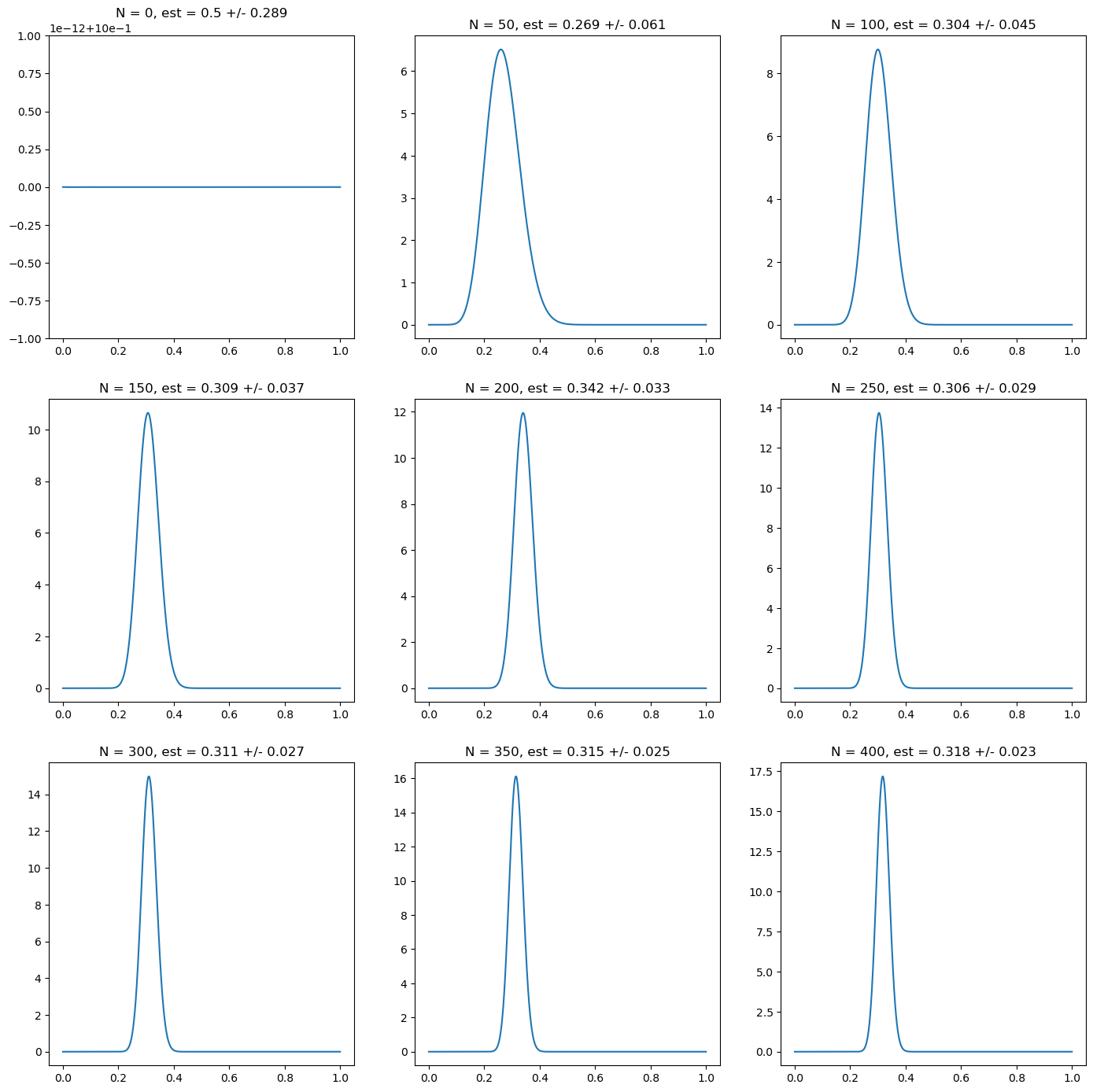
Fig. 5.1 Posterior probability for the probability of heads on a random simulation of a coin with underlying probability \(p_H = 0.3\). Every subplot corresponds to 50 new observations. The first one corresponds to the prior, in this case a uniform one: \(\alpha = \beta = 1\) in the Beta distribution prior. We characterize the posterior probability using the mean and the standard deviation of the posterior probability.#
A similar result is achieved using Jaynes’ non-informative prior, as shown in the next figure. This is achieved by taking the limit \(\alpha, \beta \rightarrow 0\), i.e. zero effective prior observations. Despite the strong bias towards the extreme values of the distribution, this does not prevent that the posterior incorporates quickly the information from the observations, at the same rate as the uniform prior in this numerical simulation.
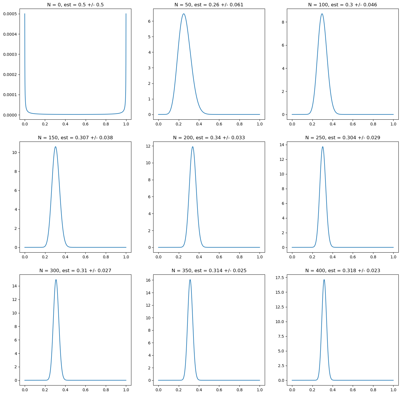
Fig. 5.2 Posterior probability for the probability of heads on a random simulation of a coin with underlying probability \(p_H = 0.3\). Every subplot corresponds to 50 new observations. The first one corresponds to the prior, for which we choose a non-informative one for this simulation, which we proxy using \(\alpha = \beta = 10^{-6}\). We characterize the posterior probability using the mean and the standard deviation of the posterior probability. Despite the strong biased towards the extremes, this choice does not affect the speed of convergence towards the true value.#
Finally, we use a prior that contains meaningful prior information, albeit erroneous one, since the prior distribution assumes that \(p_H\) has a mean value of \(0.5\) with a standard deviation of \(0.064\). This corresponds to a Beta distribution with \(\alpha = \beta = 30\), which we interpret as 60 effective prior observations. In this case, a larger number of real observations is required to override the effect of the prior. For instance, with \(50\) observations the estimation is still half way between the prior one and the real one in this simulation. For \(400\) observations, the estimation is still influenced by the prior. It takes around \(1000\) observations to converge to the real value.
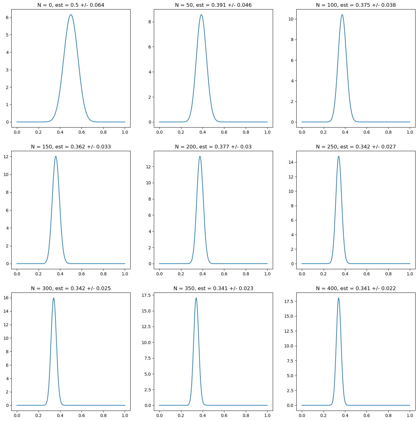
Fig. 5.3 Posterior probability for the probability of heads on a random simulation of a coin with underlying probability \(p_H = 0.3\). Every subplot corresponds to 50 new observations. The first one corresponds to the prior. In this case, we choose a prior relatively confident of a value of \(0.5\) for \(p_H\), corresponding to a choice \(\alpha = \beta = 30\). We characterize the posterior probability using the mean and the standard deviation of the posterior probability. The plots show a slow convergence to the true value due to the effect of the prior information into the estimation.#
Such result could suggest that is always better to choose non-informative priors given the penalty of using wrong prior information. However, as shown in the following figure, having good prior estimation can speed up the process of learning with respect to the case of using non-informative priors. We choose in this case a prior with \(\alpha = 18, \beta = 42\), which corresponds to a prior mean of \(0.3\) and standard deviation \(0.059\). This choice corresponds to the same number of effective prior observations as the previous case, to provide a meaningful comparison.
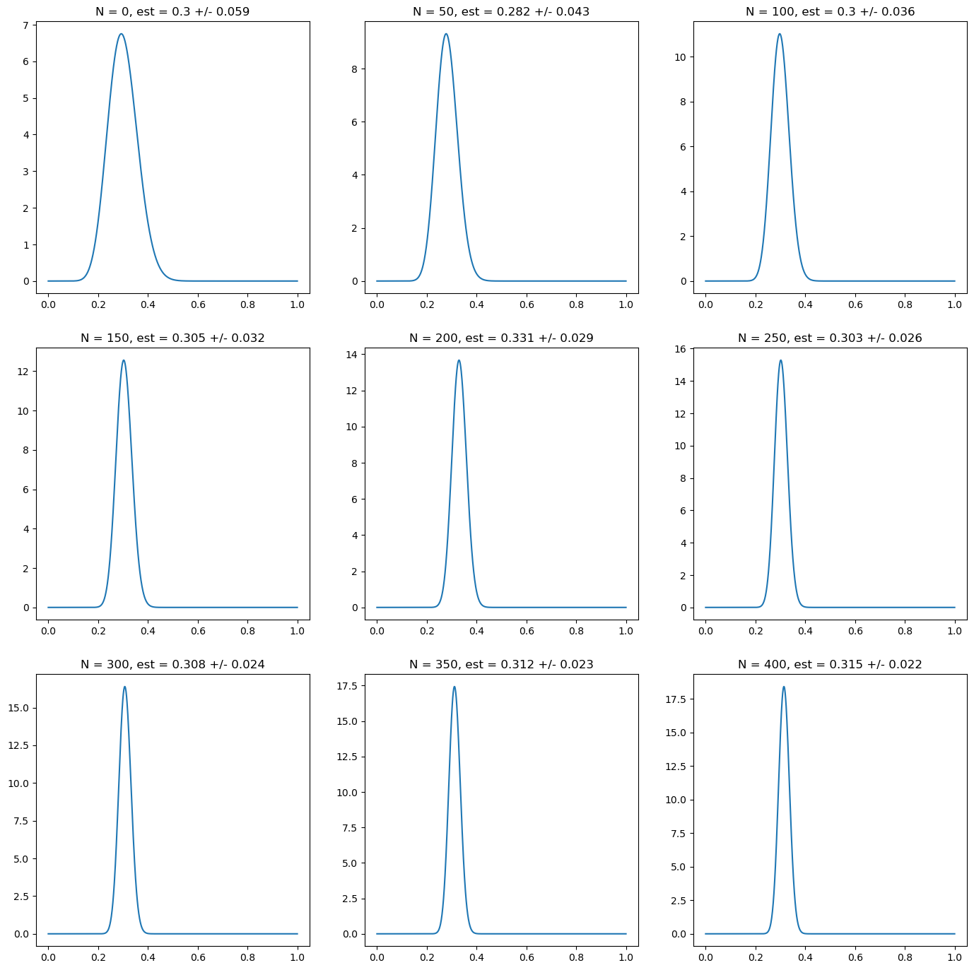
Fig. 5.4 Posterior probability for the probability of heads on a random simulation of a coin with underlying probability \(p_H = 0.3\). Every subplot corresponds to 50 new observations. The first one corresponds to the prior, which in this case has a correct prior belief on the value of \(p_H\). This corresponds in this case to a choice \(\alpha = 18, \beta = 42\). We characterize the posterior probability using the mean and the standard deviation of the posterior probability. The plots show a quick convergence to the true value with high confidence.#
5.2. Bayesian Machine Learning#
One of the main advantages of Bayesian theory is its simplicity and coherence. The toolkit presented in the previous section can be used in principle to evaluate the probability of any hypotheses conditional to the available information. In modern Machine Learning (ML), specific emphasis is placed on two families of hypotheses:
Hypotheses on the value of parameters of a given model. This is the learning task in the ML jargon. From a Bayesian point of view, as we saw in the previous section, they are simply stated as posterior distributions of parameters given the available information, in particular observations in a training set: \(P(\theta|D)\). Recall that the outcome are probability distributions. If we want to reduce parameter estimation to point estimators, Bayesian theory needs to be complemented with Decision theory.
Hypotheses on the future value of observations. This is the prediction task in the ML jargon. In Bayesian theory, this can be again written in terms of a posterior probability, in this case on the values of unobserved data \(\bf{x}\) given the available observed data: \(P({\bf x}|D)\)
Bayesian Machine Learning is therefore an application of Bayesian theory to the hypotheses of interest in Machine Learning, namely learning and prediction. Let us have a closer look to them.
5.2.1. Bayesian learning#
As mentioned, in Bayesian theory, learning from data is a result of the application of the Bayes’ theorem to an existing prior probability distribution. In terms of Machine Learning problems, it can be applied both to supervised learning problems, where we model the probability of a target \(t\) (continuous in regression, discrete in classification) conditional to a set of features \(\bf{x}\) and some observed data \(\it{D}\):
or to unsupervised machine learning problems, where we model the probability of a data point \(\bf{x}\) given some observed data \(\it{D}\):
We start by modelling these probability distributions with a prior distribution, specified by a set of parameters \(\bf{\theta}\). Recall that in the Bayesian paradigm, these parameters are also modelled with a probability distribution, whose prior is:
where \(\bf{\alpha}\) are hyper-parameters of this prior distribution. Now we observe some data \(\it{D}\) which includes observations of the target and the features. Bayesian learning means updating the distribution of the parameters that define the predictive distribution after observing new data, i.e.:
In general, the posterior distribution of the parameters will not have a closed-form, due to the difficulty of computing the denominators (the evidence). There are typically four approaches to tackle this problem:
As we saw in the previous section, in the particular case where we use conjugate priors, the posterior can be computed analytically. For a conjugate prior, the posterior belongs to the same to the same family of distributions as the prior, with updated parameters.
Laplace approximation: in this case the posterior distribution is approximated by a Gaussian by using a second order expansion of the log probability of the posterior around its maximum (MAP, Maximum a Posteriori). We will discuss it later in this section
Monte Carlo methods, which aim to generate samples from the posterior distribution, despite not having a closed form. In particular, Markov Chain Monte Carlo (MCMC) methods are the most popular ones, which rely on building a Markov Chain that asymptotically converges to the posterior.
Variational methods, which seek to analytically approximate the posterior by finding the closest one from a more simple family of distributions (e.g. Gaussian ones). For a distance between distributions, the Kullback–Leibler divergence is typically used. A particular case of a variational methods is that of Mean Field Theory, widely used in Statistical Physics, in which the posterior distribution is approximated by the distribution of a set of independent latent factors.
For an introduction to the most computational demanding methods like MCMC and Variational Methods, a good starting reference is [ONLINE BAYESIAN BOOK]
5.2.1.1. Bayesian online learning#
Bayesian learning is particularly suitable for online (or mini batch) learning. In this case, the prior distribution is the result of previous learning, and the posterior updates this prior as new data arrives. In the strictly online limit, this means every time a new observation arrives. Formally, this means:
where \(\it{D}_t = \{\it{d}_t, \it{d}_{t-1}, ..., \it{d}_0\} = \{\it{d}_t, \it{D}_{t-1}\} \) represents the dataset indexed by the time \(t\) of arrival of new information, being \(\it{d}_t\) the data acquired at time \(t\).
5.2.2. Bayesian prediction#
After observing some data and updating the probability distribution of the parameters of the model, the model can be used to perform inferences in supervised and unsupervised problems. The peculiarity of the Bayesian Machine Learning paradigm is that we don’t have a single predictive model, but a family of them parametrized by \(\bf{\theta}\). By learning we aim to narrow down which of the possible models within this family explain better the observed data. But in contrast to classical statistics, we don’t need to narrow our choice to one of these models (like the most likely one), but we use the whole posterior distribution over parameters to improve predictions.
In the supervised machine learning problem, this translates in the following predictive distribution for the target:
Similarly, in the unsupervised machine learning problem, the distribution of the target data given observations is calculated as:
These integrals are typically difficult to solve, except for some particular choices for the family of distributions. In case the integrals are intractable, one can resort either to numerical approximations or analytical ones.
Among the analytical approximations, the most simple one is using the MAP (*Maximum a Posteriori+) solution, which as discussed in the previous section means calculating the most likely value of the parameters using the posterior distribution:
Then we do the approximation:
and therefore:
An improvement upon this approximation is using the Laplace approximation for the posterior, which essentially consists on approximating the posterior using a second order Taylor series around the MAP estimator. Instead of dealing, though, directly with the posterior, it is better to work with its logarithm \(L\). For simplicity, let us consider the case of a single parameter to estimate:
where the first order term is zero since we are expanding around the maximum, and the second derivative is negative. The Laplace approximation for the posterior then reads:
which is a Gaussian distribution. The predictive distribution in this case cannot be derived generally, it will depend on the shape of the likelihood function.
Notice that in both approximations we are assuming that we are dealing with uni-modal distribution. In case of multi-modal distributions, these approximations no longer approximate well the posterior, and other techniques must be used.
5.2.3. Example: coin toss experiment#
Let us come back to our previous example of estimating the probability of a coin toss resulting in heads or tails. By using a Beta conjugate prior to the likelihood, the posterior had a closed-form which is an updated Beta distribution:
With the information available so far, we want to predict the result of the next coin toss. The predictive distribution reads:
which in this case is the mean of the Beta distribution. Notice that this is not the same result that we would obtain in classical statistics using maximum likelihood even if we had a uniform prior (\(\alpha = \beta = 1\)), since the mean and the mode of the Beta distribution don’t coincide, the mode being \(\frac{\alpha - 1}{\alpha + \beta - 2}\) for \(\beta > 1\)
In this case, due to the choice of a conjugate prior, we have a closed-form for the posterior and the predictive distribution can also be analytically calculated. However, let us assume this is not possible and use the Laplace approximation to obtain the predictive distribution. The MAP estimator for the posterior is, by finding the maximum of the Beta distribution:
The second order derivative of the log-likelihood evaluated at the maximum MAP then reads:
The posterior distribution is therefore approximated by the following Gaussian distribution:
The predictive distribution is now easy to evaluate since it is just the mean of a Gaussian:
The result differs slightly from the exact one, but for \(N, n_H >> 1\) and / or \(\alpha, \beta >> 1\) they converge, as it is actually expected since in this regime the Beta distribution has the Gaussian distribution as a limit, as discussed in the previous section.
We can test the validity of this result numerically by plotting the actual posterior and the Laplace approximation, for different number of observations and specification of the prior:
CONTINUE
5.3. Bayesian Linear Regression#
5.4. Probabilistic Graphical Models#
5.5. Latent variable models#
So far we have been working with probabilistic models where all variables are observable. Latent variable models are probabilistic models where some of the variables cannot be measured or can only be partially measured, i.e. there is missing data in some of the records of the dataset.
In both cases, formally we define latent models as a probability distribution over two sets of variables:
where \({\rm x}\) are the set of observable variables and \({\rm z}\) the latent ones. \(\theta\) are the parameters of the probability distribution, which we state explicitly for convenience later.
5.5.1. Partially observable latent variable models#
As mentioned above, in this case we are dealing with a problem of missing data, where some of the data points of a set of variables have not been recorded for potentially various reasons. Rubin [1] distinguishes between tree different situations regarding the generative model (i.e. the full probability distribution) for missing data:
Missing Completely at Random (MCAR): there is no pattern in the missing data. The missing data is uncorrelated with observed and unobserved data. For instance, if some trades in a booking database are missing due to corruption of the physical support.
Missing at Random (MAR): in this case there is pattern in the missing data that can be explained using observed data. Coming back to the example of a trades database, if the missing data is due to a particular sales person that tends to forget to register a voice operation in the systems
Missing Not at Random (MNAR): in this case there is also a pattern in the missing data, but can only be explained using unobserved data (e.g. full latent variables). In the example of the booking database, if the issue comes from a certain sales person as in MAR, but the booking database does not record in any case the sales person identity.
The use of probabilistic methods for missing data is called multiple imputation and is described extensively in [1]. The idea is essentially to estimate the model from the observed data using the techniques we will explore below in this section, and use it as a generative model for the unobserved variables, namely computing:
Imputation of missing data can then be done using some statistic of the distribution like the mean or the median, or generating random samples from the distribution.
Multiple imputation works well for MCAR and reasonably (with some negligible bias) for MAR. The case of MNAR is more complicated, and can only be properly dealt with by introducing full latent variables that properly capture the MNAR mechanism, which is difficult if there is not a prior knowledge of the missing data mechanism.
5.5.2. Full latent variable models#
In this case, there are not available observations of the latent variables. Models with full latent variables are closely related to probabilistic graphical models, since in many situations latent variables are introduced as prior knowledge in the structure of a model about a certain process, particularly when trying to model causal relationships. For instance, a model of two variables that are correlated but we believe not to be directly causally related, can be naturally extended by introducing a latent variable, a confounder, that influences both.
We can distinguish between two practical cases where latent variable models naturally emerge:
On the one hand, in problems where we know of the existence of a relevant variable, but it has not been observed and recorded in the data gathering process. An example, for instance, in the problem of demand estimation where only trades are observed, are the total interests or requests from clients to trade, that only in a fraction of cases (the hit & miss) generate a trade.
On the other hand, a latent variable can be an abstraction that cannot be directly measured but it might represent a common influence or effective factor.
One example is that of a market regime, which is modelled as a categorical variable with a set of states (e.g. high volatility and low volatility), and influences the price returns. Hidden Markov Models are latent variable models frequently used to model the effect of so-called regime switch of the statistics of price returns. They are typically applied as signal generators that alert of changes in market behavior.
Another example is the concept of mid or fair price. In real markets price information comes from trades, RfQs, limit order books, composite prices and so on. But the concept of mid / fair price of an instrument is unobservable. Kalman filters are typically used to infer the value of the mid-price from price informative observations.
5.5.3. Examples of Latent Variable Models#
5.5.3.1. Gaussian Mixture Models (GMMs)#
The Gaussian Mixture Model postulates that data observations \(\vec{x}_n\), \(n = 1, ..., N\) are generated by \(K\) independent multivariate Gaussian distributions with unknown parameters \(\vec{\mu}_k, \Sigma_k\). The membership of each data point to a particular Gaussian is determined by latent categorical random variables \(z_n = {1, ..., K}\) with probabilities \(\pi_k\). Gaussian Mixture models are used to model unobserved subpopulations or segments from a given population. The probability distribution is therefore given by:
which is a linear combination of Gaussian distributions, hence the name mixture of Gaussians. Mixture models are actually more general in that other distributions can be used to model the mixture components, namely a Binomial, Dirichlet, Poisson, Exponential, etc.
As a graphical model, the so-called plate notation is usually employed to simplify the representation of the \(N\) random variables \(\vec{x_n}\) and their associated \(K\) latent random variables \(z_n\) categorizing their mixture component membership. The following figure represents the mode in plate notation:
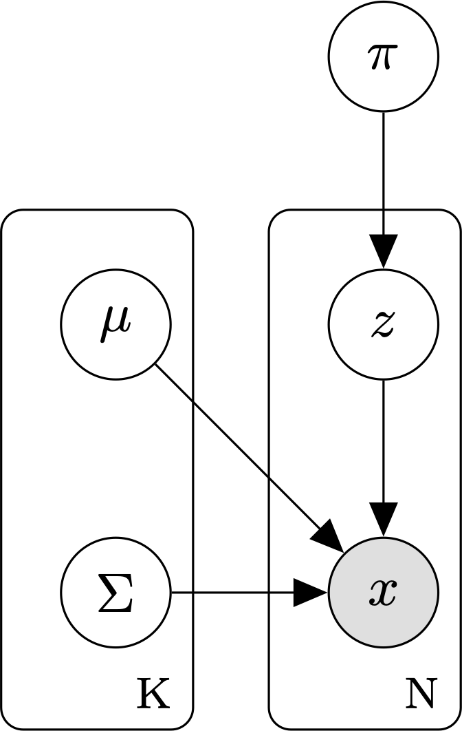
Fig. 5.5 Gaussian Mixture Model in plate notation.#
The joint probability distribution of the model, including the latent variables, is the following:
where \(\delta_{z_n,k}\) is an indicator function: \(\delta_{z_n,k} = 1\) if z\(_n = k\), \(0\) otherwise
Gaussian mixture models have plenty of real-life applications. The most popular probably is its use as a clustering technique, and actually the most popular clustering technique itself, K-Means, is a particular case of the Gaussian Mixture model for spherical distributions, \(\Sigma_k = \epsilon I\), in the limit \(\epsilon \rightarrow 0\), when it is calibrated using the Expectation Maximization (EM) algorithm (see section below).
Another interesting application is anomaly detection, particularly for one-dimensional data. If we have theoretical reasons to expect the distribution of data to be a Gaussian, we can use a mixture of two Gaussians distributions with the same mean but different standard deviations to capture anomalies from normality:
where \(G\) and \(B\) stand for good and bad, respectively, since the model is called the Good and Bad data model [2]. After learning the parameters of the model using our data (\(\pi_G\), \(\mu\), \(\sigma_G\), \(\sigma_G\)), and making by definition \(\sigma_B \geq \sigma_G\), we classify as anomalies those points in the dataset that are more likely to have been generated by the “bad” data Gaussian. This is done by inferring the probability of being “bad data” using Bayes’ theorem:
and classifying as “bad data” or anomalies those points whose probability exceeds a given threshold, typically 0.5. This anomaly detection model works surprisingly well highlighting anomalies in data that humans could also recognize visually, making it a good candidate for automating human-driven anomaly detections.
5.5.3.3. The Kalman Filter#
A Kalman filter is a particular instance of a filtering algorithm first proposed by Rudolf E. Kalman in 1960 in his seminal paper “A New Approach to Linear Filtering and Prediction Problems” [4]. It is a particular case of a Hidden Markov Model where both the hidden and observed variables are continuous and follow Gaussian distributions. In this simple case, inference and learning becomes tractable, making it a very efficient estimation algorithm. Actually, the term Kalman Filter applies rigorously to an estimation algorithm that takes a series of noisy observations and produces estimations of the underlying variable by combining its previous estimate and the current observation. In order to be optimal, transition and observation noises have to be Gaussian.
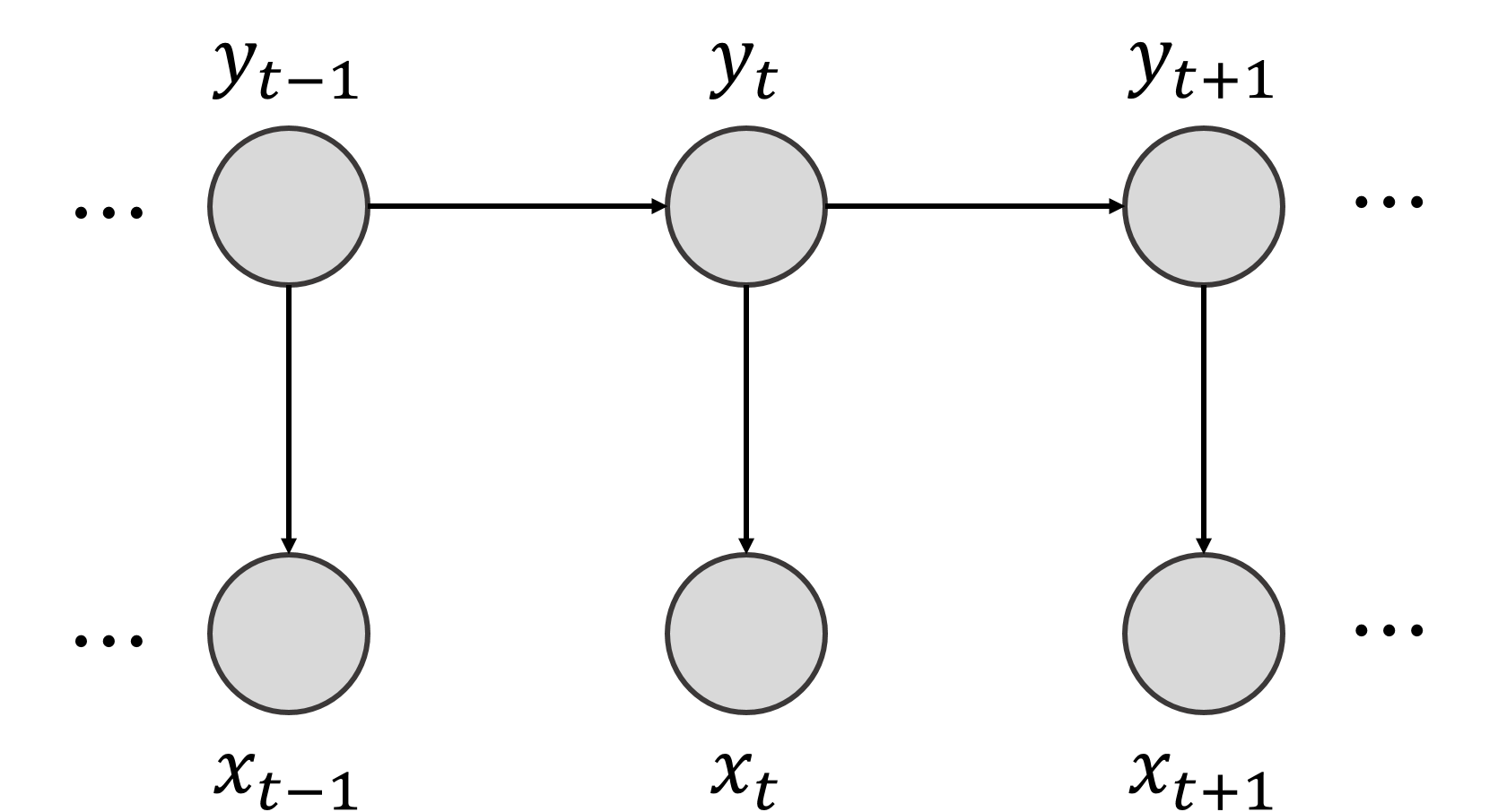
The model in its graphical form is the same as shown in the HMM, being a particular case of this one. Mathematically, and considering for generality a vector of observations and hidden states, it can be written as:
The Kalman Filter is a recursive algorithm to estimate the hidden state value given observations, using two steps: the prediction and the update. First, using the best estimate at \(t-1\), we predict the value of the hidden state at \(t\) and its covariance \(P\):
where we use the suffix \(\{t|t-1\}\) to distinguish between the optimal estimations and the underlying random variables. Then, given an observation at \(t\), we update the estimation as:
where \(K_t\) is called the Kalman gain. It controls the impact of the observation on the final estimate: if \(K_t = 0\), then the final estimation is purely the prediction, whereas for \(K_t = I\), the estimation is fully determined by the observation.
These so-called filtering equations can be derived using probability theory, computing the posterior distributions under the information available. For the predict step, this means computing:
where \(\vec{x}_{0:t}\) denotes observations up to \(t\). For the update state, we compute:
i.e. now we include the observation at time \(t+1\) to update the estimation of the latent variables.
The filtering equations are central to Kalman filtering, as in most applications the goal is to estimate the most recent values of the latent variables given all available information up to the current time. However, there are situations where we may want to refine estimates of latent variables at earlier times by incorporating all available information, including observations collected after the time of interest. In such cases, the quantity of interest is
where information up to time \(T\) is taken into account. The equations derived for this inference are known as smoothing equations, since the refinement produces a smoother estimate of the latent variables across time.
In the next subsection, we will derive both the filtering and the smoothing equations computing these probability distributions for a simple instance of the Kalman filter: the local level model.
Kalman filters have many applications in multiple domains. In financial markets, they can be used to combine different noisy observations of spot prices to infer a consistent estimate of a fair or mid price, to be used typically in the market-making of relatively illiquid instruments like bonds or some derivatives [5]. Another use case is to infer prices of instruments when markets are closed, which can be useful for hedging indexes that have components with different time zones. In reference [6], they have been applied to the estimation of term structure models. And in the context of investment strategies, they have a relatively popular application to improve pairs trading strategies [7]. We will delve into some of these applications later in this book.
5.5.3.3.1. The local level model#
A simple tractable model that illustrates well the general theory of the Kalman filter is the local level model, which despite its simplicity can have relevant applications, for instance in pricing. The model has the structure:
Derivation of the forward filtering equations: predict and update
The predict equation can be derived by computing the distribution of \(y_{t+1}\) conditional to the previous observations, which we denote \(x_{0:t}\):
We can compute this probability by using the marginalization rule over the latent variable \(y_t\):
where we have exploited the graphical structure of the model to simplify \(p(y_{t+1}|y_t, x_{0:t}) = p(y_{t+1}|y_t) = {\mathcal N}(y_{t+1}| y_t, \sigma_w^2)\), since \(y_t\) is the only parent of \(y_{t+1}\). The proof is based on induction: let us assume that \(p(y_t|x_{0:t}) \sim {\mathcal N}(\hat{y}_{t|t}, \sigma_{t|t}^2)\), i.e. it is Gaussian with mean \(\hat{y}_{t|t}\) and standard deviation \(\sigma_{t|t}\). \(p(y_{t+1}|x_{0:t})\) is therefore the result of the convolution of two Gaussian distributions, which is itself a Gaussian distribution with:
This completes the derivation of the predict equations, given by:
where, as a reminder to the reader, we use the notation \(t_1 | t_2\) to mean a variable at time \(t_1\) conditional to information up to \(t_2\). We have not yet, though, completed the induction proof, since we have not proven why \(p(y_t|x_{0:t})\) follows a Gaussian distribution.
This is directly linked to the derivation of the update equation, which corresponds to the following inference:
We can write \(p(y_{t+1}|x_{0:t+1}) = p(y_{t+1}|x_{0:t}, x_{t+1})\) and apply Bayes’ theorem on \(x_{t+1}\):
We readily recognize the probability distribution derived in the predict step:
Moreover, from the model definition we have:
This is the normalized product of two Gaussian density functions, which is also a Gaussian density function, since we can complete the square:
where we have omitted terms that are constant with respect to \(y_{t+1}\) and we have defined:
If we introduce the Kalman gain as:
we can write these equations as:
which are the update equations of the Kalman filter, corresponding to the mean and variance of \(y_{t+1}\) conditional to observations up to \(t+1\), which follows a Gaussian distribution:
As a consequence, we have proven by induction that \(p(y_t|x_{0:t})\) follows a Gaussian distribution, as long as the initial condition \(p(y_0)\) is also Gaussian.
Derivation of the smoothing equations
The derivation of the smoothing equations follows the same lines as the forward filtering equations. In this case, we are interested in computing:
i.e., we seek to infer the distribution of the latent variable at \(0 \leq t \leq T\). We can exploit the structure of the graphical model to compute this expression by conditioning on \(y_{t+1}\):
Where we have used, in the second step, the fact that conditioning on \(y_{t+1}\) removes the dependence on \(x_{t+1:T}\).
We assume that we have already done the forward filter path, so we have computed the distributions \(p(y_t|x_{0:t}) \sim {\mathcal N}(\hat{y}_{t|t}, \sigma^2_{t|t})\) and \(p(y_{t+1}|x_{0:t}) \sim {\mathcal N}(\hat{y}_{t+1|t}, \sigma^2_{t+1|t})\). In particular, notice that for \(t = T\), the filtering and smoothing inferences are the same, given by \(p(y_{T}|x_{0:T})\).
Therefore, we will derive the smoothing equations backwards starting from \(p(y_{T}|x_{0:T}) \sim {\mathcal N}(\hat{y}_{T|T}, \sigma^2_{T|T})\) as the initial condition. The key idea is to assume that we already have computed:
and use it to compute \(p(y_t|x_{0:T})\). This means to compute the previous integral which depends on \(p(y_{t+1}|x_{0:T})\) which we have already computed, and \(p(y_t|y_{t+1}, x_{0:t})\), which we need to derive. We use the standard trick of computing the join probability \(p(y_t, y_{t+1}|x_{0:t})\). Since \(y_{t+1} = y_t + w_t\), where \(y_t\) and \(w_t\) are uncorrelated, this is simply:
where we have used that \(cov(y_t, y_{t+1}) = var(y_t)\) in this model. Now we can derive the conditional distribution using:
Computing this expression we get:
Now we have the expression for the two probabilities involved in the calculation of \(p(y_t|x_{0:T})\), which can be carried by completing the squares on \(y_{t+1}\) and integrating it away. The final result is, unsurprisingly, a Gaussian distribution with the following backward iterative equations for the mean and variance, which conform the Rauch - Tung - Striebel smoothing equations:
As mentioned, we compute first the forward filtering equations until \(T\), which are used to initialize the smoothing equations and proceed backwards. The smoothing equations provide a better estimation than the filtering ones, since they use the full information set up to \(T\). This translates into smaller estimation variances. They cannot be used in an online context, though, which is where Kalman filters find a large number of applications. Their main application is parameter estimation, since they are required to compute the likelihood of the data when using maximum likelihood estimation.
5.5.4. Estimation of Latent Variable Models#
Given observations and a latent variables model typically represented as a probabilistic graphical model, we would like to estimate the parameters of the model. The difficulty, here, comes from the latent variables, for which we don’t have observations. There are different ways to estimate parameters in this case, but we will focus on the most popular ones: maximum likelihood estimation (MLE) and expectation maximization (EM), which computes an approximation of the MLE solution.
5.5.4.1. Maximum Likelihood Estimation (MLE)#
The presence of latent variables does not preclude the use of MLE. Our goal is still to find the parameters that maximize the probability of the observations given the parameters (or likelihood). If we could observe the latent variables, that would mean maximizing the so-called (in the context of latent variable models) complete likelihood:
Sine the latter are not observed, we need to integrate them out:
where we have assumed discrete distributions for the latent variables. For continuous ones, the sums have to be replaced by integrals. The latter is called the incomplete likelihood.
Whereas maximizing incomplete likelihoods with respect to the parameters is in theory possible, in practice it is usually a computationally expensive method. Therefore the need to develop more efficient estimation methods like Expectation Maximization.
5.5.4.2. Expectation Maximization (EM)#
If we were to have observations of the latent variables, we could then maximize the complete likelihood and get maximum likelihood estimators for the parameters \(\theta\). However, we don’t have those observations and we need to maximize the incomplete likelihood, which is a harder problem.
The intuition behind the Expectation Maximization (EM) method lies in this idea of maximizing the complete likelihood. Since we don’t have observations of the latent variables, EM seeks to maximize the incomplete likelihood breaking the problem in two easier steps:
E-step: use observations and current best estimates of the parameters to infer values for the latent variables
M-step: Plug these values into the complete likelihood and maximize it to get new estimations for the parameters These steps are repeated until convergence.
Mathematically, EM does not guarantee to find a global optimum for the incomplete likelihood, but under certain general conditions it can be shown that the EM solution is a lower bound for the global maximum.
Let us now look at the algorithm in more detail. We start with the E-step. The best estimate for the hidden variables given the latest estimation of parameters \(\theta^{(s)}\) and observations is given by the following conditional distribution:
It is called E-step because it computes the expectation of the complete (log)likelihood (the log to make it easier to compute) using this distribution, where the complete log-likelihood has yet unknown parameters \(\theta\), which we denote:
where we have introduced the compact notation \(\mathbb{E}_s[...] = \mathbb{E}[...|\{{\rm x_n}\},\theta^{s}]\).
The M-step then maximizes this function with respect to \(\theta\), which become \(\theta^{(s+1)}\) in the iterative algorithm.
The sketch to prove that the EM solution is a lower bound of the maximum incomplete likelihood is relatively easy, so we do it in the follow. We start from the incomplete log-likelihood:
where \(q(z_n|x_n)\) is so far a generic distribution. Now since \(log\) is a concave function, we can use Jensen’s inequality, whose general form is:
where \(\lambda_n \geq 0\) and \(\sum_n \lambda_n = 1\). Applied to our case, where \(\lambda_n = q({\rm z_n}|{\rm x}_n)\):
with \(F(q,\theta)\) is called the free energy in analogy of Statistical Mechanics. The free energy is therefore a lower bound of the incomplete likelihood:
If we maximized the free energy we are optimizing a lower bound of the incomplete likelihood, which is essentially what we claim EM does. EM maximizes the free energy using coordinate gradient ascent, i.e. iteratively optimizing \(F\) in \(q\) and \(\theta\):
E-step: \(q_{s+1} = {\rm argmax}_q F(q, \theta^{(s)})\)
M-step: \(\theta_{s+1} = {\rm argmax}_\theta F(q_{t+1}, \theta)\)
To finish the proof, we only need to find the solution for the E-step. A simple proof consists in first noticing that the inequality also holds for \(\theta = \theta^{(s)}\):
Now let us take \(q_{s+1} = P(z_n | x_n, \theta^{(s)})\). Plugging it in into the free energy:
which makes the inequality an equality, therefore maximizing the free energy!
For the M-step, we just need to sustitute \(q_{s+1}\) into the free energy:
where the second term, \(H_{q_{s+1}}\), the entropy of \(q_{s+1}\), does not depend on \(\theta\). Therefore the maximum of this free energy wrt to \(\theta\) is the same as the maximum of \(Q\):
completing the proof.
The algorithm is run until some form of convergence is reached (or a maximum number of iterations). Two different criteria are used typically to evaluate convergence:
Convergence in the incomplete log-likelihood \(l(\theta^{(s)})\), which we now from the previous proof that has to increase always on each EM iteration. The only issue is that potentially might be computationally expensive to evaluate, since it requires the integration over the latent variables.
Convergence in parameters, meaning that two subsequent set of parameters are close enough using some distance metric, for instance Euclidean distance:
In the following examples we will see examples of a general rule when using EM, namely that the estimators of the parameters \(\theta\) obtained in the M-step are the ones that we would get by optimizing the incomplete likelihood but with the values of the latent variables replaced by their expectations under \(P(z_n | x_n, \theta^{(s)})\)
5.5.4.2.1. Example 1: Gaussian Mixture Model#
As a first example we derive EM for the Gaussian Mixture Model (GMM). The complete log-likelihood for this model reads:
The set of parameters \(\theta\) of the model are the segment probabilities \(\pi_k\) and Gaussian parameters \(\vec{\mu}_k, \Sigma_k\). Given observations \(\vec{x_n}\) and a current estimation of parameters \(\theta^{(s)}\), where \(s\) is the index for the current EM iteration, we infer the distribution of the latent variables (E-step):
where we have used Bayes theorem. Now we write the expected log-likelihood with respect to this distribution, which again for simplicity of notation we denote as \(\mathbb{E}_s[...]\):
Now we apply the M-step, finding the estimators for the parameters that maximize the expected log-likelihood. For the case of \(\pi_k\) we need to introduce the constraint \(\sum_k \pi_k = 1\):
Similarly we can find the estimators for the Gaussian parameters:
From these estimators, we can easily verify that indeed they are of the form of the estimators we would obtain for the complete log-likelihood, but with the hidden variables replaced by their expectations under the posterior \(P(z_n=k|\vec{x}_n, \theta^{(s)})\). Another interesting point to remark is how the EM algorithm for the GMM is essentially a “soft” version of K-means, where instead of having hard assignments to the cluster with the nearest centroid, we have soft assignments to each of the Gaussian distributions. We left to the student the task, as an exercise, to show how EM converges to K-means in the particular case of spherical distributions \(\Sigma_k = \epsilon I\) in the limit \(\epsilon \rightarrow 0\).
Let us now illustrate the algorithm in practice. We apply the Good and Bad Data Model (GBDM) to detect anomalies in the daily returns of BBVA stock.
The intuition behind GBDM is that, under normal market conditions, price returns approximately follow a Gaussian distribution, consistent with the Geometric Brownian Motion (GBM) model for stock prices first proposed by Samuelson. Yet, it is well established that financial markets can experience episodes of extreme stress in which returns deviate sharply from the predictions of GBM—for example, during the COVID-19 confinement, the Brexit referendum, or the first election of Donald Trump. The GBDM captures these empirical features by combining two components: a Gaussian distribution representing the good regime of normal market behavior, and a second Gaussian distribution accounting for the bad regime of stressed conditions. In this way, the model provides a simple but powerful generative framework for distinguishing between typical fluctuations and anomalous events in financial time series.
Specifically, we consider a fixed 10-year window, compute daily returns, and fit the model to this time series using the Expectation–Maximization (EM) algorithm. For initialization, we set the mean of the historical returns as the common mean of both the good and bad data components. The standard deviation of the good data distribution is initialized with the historical standard deviation of returns, while the bad data distribution is initialized with twice this value. As a prior probability, we assume that 95% of observations belong to the good regime. Importantly, the final results are quite robust to these initialization choices, which suggests that the model reliably captures the distinction between normal and anomalous returns.
We check that the EM algorithm behaves as expected, i.e. the incomplete log-likelihood always increases with each iteration of the algorithm, and it reaches convergence. This is shown in the following figure:
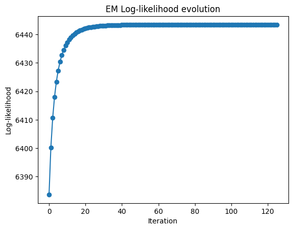
Fig. 5.7 Log-likelihood of the GBDM calculated with the parameters obtained at each iteration. As expected from the theoretical formulation of the algorithm, the log-likelihood cannot decrease at any iteration of EM.#
To classify anomalies, we use a \(P(\text{bad}|D) > 0.5\) rule to classify data as abnormal. In the following two figures we can see the results of the model in both the histogram and time-series of daily returns of BBVA. The GBDM partitions the data in two clusters: one that captures normal financial conditions, and a second one that flags periods of stress as well as exuberance (abnormally high negative and positive returns, respectively). By inspection of the data in the accompanying notebook we can see that the model correctly classifies the aforementioned events, since it flags the 2020-03-16 (the first lock-down day in Spain), the 2016-06-24 (the first trading day after the Brexit referendum) and the 2016-11-09 (the first trading day after Trump’s election).
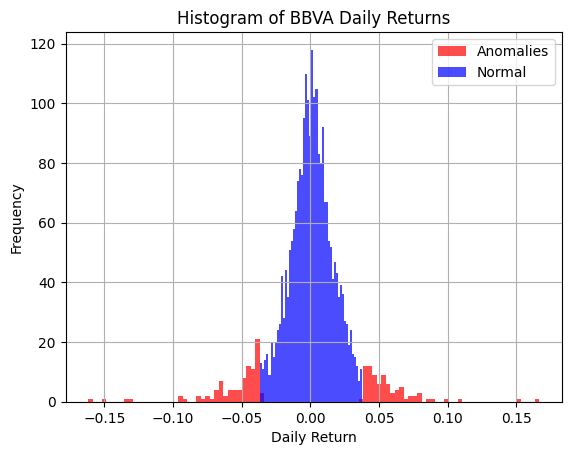
Fig. 5.8 Histogram of daily returns of BBVA’s stock over 10 years from 2015 to 2025. The GBDM model has been used to flag anomalous returns, which are depicted in red.#
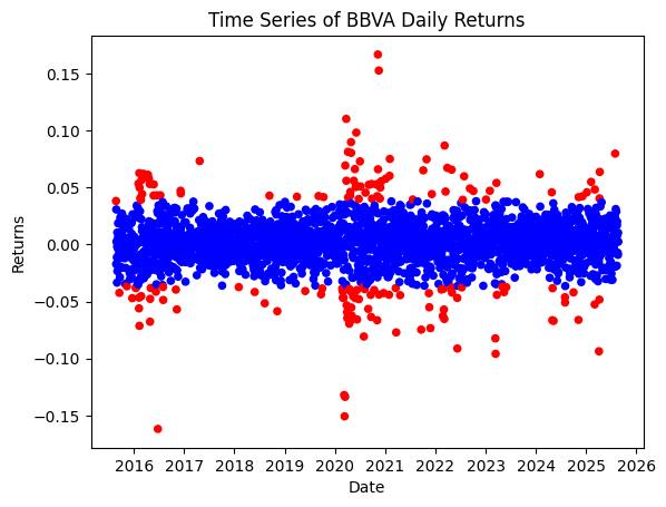
Fig. 5.9 Time-series of daily returns of BBVA’s stock over 10 years. Again, red points depict days that have been classified as having abnormally high and low returns.#
5.5.4.2.3. Example 3: Local Level Model (simple case of a Kalman Filter)#
Recall that the local level model equations are given by:
Assume we have observations \(x_{0:T}\). The complete log-likelihood is similar to the one for the HMM, only now we exploit the properties of the Gaussian distributions:
As usual with EM we derive the iterative equations using induction: we assume we have already a set of parameters estimated at iteration \(s\), \(\theta^{(s)} =\{\sigma_v^{(s)}, \sigma_w^{(s)}\}\) and derive the updates for iteration \(s+1\). To initialize the algorithm we need a parameter seed that can be based on general heuristics or prior information. We start with the E-step, where we compute the expectation of the log-likelihood using the best inference available on the latent variables at the current iteration, \(P(y_t|x_{0:T}, \theta^{(s)})\):
where \(\mathbb{E}_s[...] \equiv \mathbb{E}[... |x_{0:T}, \theta^{(s)}]\). Let us compute the first of the expectations:
where we have used the smoothing equations introduced previously, only their iterative computation is done using parameters \(\theta^{(s)}\). The second one can be computed as:
where we have introduced the smoothed estimation of the one-lag covariance \(\sigma_{t+1,t|T}^{(s)} \equiv \mathbb{E}_s[y_{t+1} y_t] - \hat{y}_{t+1|T}^{(s)} \hat{y}_{t|T}^{(s)}\). A derivation of the recursive equation to compute this covariance can be checked in [3]:
where we have introduced the smoother gain \(J_t\):
Let us move now into the M-step, where we obtain new estimators for the parameters of the model by maximizing the expected complete likelihood. We compute the extremes and leave the interested reader the evaluation of the second derivatives to verify that they are indeed maxima:
The new estimators depend on the expectations calculated in the E-step, which themselves are calculated doing a forward and smoothing passes over the data.
This completes the derivation of the EM algorithm for the local level model, since now starting from a seed for the parameters, we can iteratively refine our estimators until we reach a convergence in terms of parameters or log-likelihood.
To see the algorithm in action we simulate a local level model over 200 time-steps, with \(\sigma_v^2 = 1.0\) and \(\sigma_w^2 = 0.05\). Then we use the simulated data to find the parameters using Expectation Maximization. The algorithm reach quickly convergence, as seen in the figure below. As a sanity check of the implementation, we see that the log-likelihood over EM iterations never decreases.
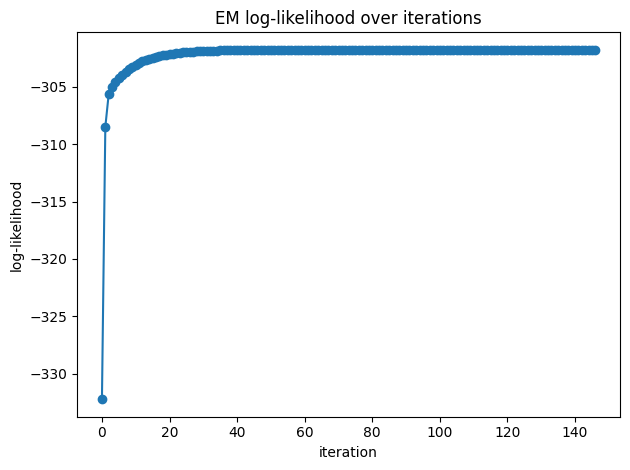
Fig. 5.10 Log-likelihood of the local level model evaluated with the estimation of the parameters using EM for each iteration. We see that log-likelihood never decreases, which is a sanity check for the correctneess of the implementation.```#
The converged parameters for this simulation are \(\hat{\sigma}_v^2 = 0.872\) and \(\hat{\sigma}_w^2 = 0.054\), which are reasonable approximations although not exact, since EM does not guarantee to reach the maximum of the likelihood. Finally, we run the smoother using the converged parameters and compare it with the observations and the true latent state variable. The smoother provides a good approximation for the true latent state, which remains within a two sigma band for the full simulation.
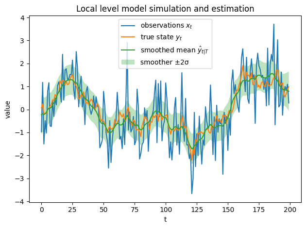
Fig. 5.11 Simulated latent state variable and observations for the local level model with \(\sigma_v^2 = 1.0\) and \(\sigma_w^2 = 0.05\). The green line shows the inferred latent state using the smoothing algorithm, with a two sigma confidence interval shaded.```#