7. Stochastic Calculus#
In this chapter we provide an introduction to Stochastic Calculus: a mathematical tool useful to build models of systems that have a relevant degree of randomness in their evolution, and such randomness is a key determinant of the properties we want to model. The latter is important: the use of Stochastic Calculus complicates the analysis of a model. It is the role of the modeller to assess initially if a deterministic model is sufficient, say because we are just interested in average properties for which randomness averages out and can be neglected. Stochastic Calculus is useful when randomness might generate a variety of outcomes, so we want to study trajectories as scenarios weighted by probability, i.e. probability distributions.
We start the chapter introducing the study of dynamical systems, focusing initially in those deterministic models that could be a sufficient starting point for the modeller. They are also usually one part of the stochastic model, which as we will see is usually decomposed in a deterministic plus a stochastic dynamics. Then we introduce the Wiener process as a building block to build stochastic models of systems with continuous dynamics. From that, we move into stochastic differential equations as well as a few useful tools to analyze them and solve the probability distributions of their trajectories. There are not many tractable stochastic differential equations, i.e. those whose distribution can be derived in closed-form. We introduce the most typical cases when it is. Finally, we close the chapter introducing jump processes, a second useful tool to model stochastic systems, in this case those that show discontinuities in their dynamics.
7.1. Modelling dynamical systems#
We model a dynamical system a a set of variables that follow a time dynamics law
where \(\{X_t\}\) is a set of external factors that influence the trajectory of the system.
The trajectory might be difficult to derive, and sometimes it is easier to derive the dynamics in small steps. Considering the case \(y = f(t)\)
where \(g(t) = \frac{df}{dt}\) and then integrate it
In the more general case where there are external factors with their own time dynamics:
Modelization can be done empirically or using fundamental laws if available, we will see examples in next section
As mentioned, the dynamics of the system might not be deterministic. In this case we need to model the source of randomness in the dynamical system, for which we use stochastic differential equations (SDE) of the form:
where \(d W_t\) is the Wiener process (Brownian motion) that will be introduced later.
7.2. Deterministic dynamical systems#
We will introduce the topic by looking at some relevant deterministic differential equations that come across in the modelization of dynamical systems.
Example: Newton’s Laws
A first example comes from Newton’s laws applied to the dynamics of particles in a gravitational field. The second law of Newton states:
We consider an object of mass m drop at initial height \(h(0)\) with speed zero. It is only subjected to the gravitational force: \(F = m g\) where g is the gravitational constant close to Earth’s surface: \(g \approx 9.81 m/s^2\). The dynamics for the speed is therefore a first order differential equation with constant coefficients:
where we have taken into account that the force is exerted in the opposite direction to which the height axis grows. This equation is simple to integrate:
since in our case, \(v(0) = 0\). The dynamics of the position reads:
which can be again be easily integrated:
These are particular examples of a general family of differential equations:
which can be simply integrated step by step by defining intermediate variables, e.g.:
Example: simple inflation targeting model
A simple model of the dynamics of inflation takes into account Central Bank interventions using monetary policy in order to adjust inflation to a given target. When inflation deviates from the target, monetary policy is used to bring it back to the target. This can be modelled using the following differential equation:
where \(\pi\) is the current level of inflation, \(\hat{\pi}\) is the inflation target, and \(\theta > 0\) is a constant that models the speed at which monetary policy takes effect. This is an example of a mean - reverting equation, a process whose dynamics is controlled by an external force that drives back the system towards a stable level (the mean).
This equation is a particular example of a general family of differential equations which we call separable, with the form
They can be solved by exploiting the separability:
Coming back to the particular example of the mean reverting equation:
The solution shows as, as expected, a trajectory for the inflation that decays to the target. The time scale for decay is independent of the size of the initial gap \(\pi_{t_0} -\hat{\pi}\), depending exclusively on \(\theta\), which is called the mean reversion speed. In analogy to the physical process of radioactive decay, which can be described by a similar equation, we can define a half-life \(\tau\), or time in which the gap is closed by half, as: \(\tau = \frac{\log }{\theta}\) Alternatively, \(1/\theta\) is the time it takes to close the gap to \(1/e \approx 0.369\)
Example: Free fall with friction
We can again resort to Newton’s laws to model the dynamics of an object in free fall in the atmosphere, where the air introduces an opposite resistance to the action of gravity. A simple model of such friction is a force proportional to the speed of the object, namely \(F = \eta v\), where \(\eta\) is a coefficient that depends on the properties of the atmosphere. Using Newton’s law, we have now:
Which is a system of two equations. We can combine it to get a differential equation on the particle’s trajectory:
which is, particularly, a second order non-homogeneous ODE with constant coefficients. A general non-homogeneous linear ODE with constant coefficients reads:
To solve this equation first we find a general solution for the homogeneous equation, and then a particular solution for the non-homogeneous one.
For the general solution of the homogeneous we can actually exploit its connection to a system of first order differential equations, an example of which we saw when introducing the problem of a particle in free-fall with friction. In general, we can define auxiliary variables \(y_i = \frac{d^i y}{dt^i}\) for \(i < n\). We get the following system:
which has the structure:
where \({\bf y} = (y_0, ..., y_{n-1})\) and A is the matrix form with the coefficients of the system of equations above. The general solution to this equation is:
This is the formal solution, but to get a workable solution we need to diagonalize the matrix A, i.e. finding \(A = C \Lambda C^{-1}\) where \(\Lambda\) is a diagonal matrix with the eigenvalues of A, and C has its eigenvectors \(\vec{w}\) as columns. One can then project the solution in the space of eigenvectors:
This is equivalent to writing:
where \({\bf c_i}\) is the ith eigenvector with eigenvalue \(\lambda_i\) and \(w_i = (C^{-1} {\bf y_0})_i\) is the projection of the initial state into the eigenvectors basis. In such basis, the dynamics is simple, driven by the exponential of its eigenvalue: \(e^{-\lambda_i t}\)
Coming back to the particle in free-fall, we can obtain the general solution of the homogeneous equation, namely:
by applying directly the ansatz \(e^{\lambda t}\):
which is equivalent to finding the eigenvalues of the matrix of the system of equations. This equation has two eigenvalues, \(\lambda = 0\) and \(\lambda = -\frac{\eta}{m}\), so the general solution reads:
A particular solution is a linear function \(h_t = \frac{m g}{\eta} t\). Therefore, the solution for the full equation is:
The speed is therefore:
Finally, by imposing initial conditions \(h_0\) and \(v_0 = 0\), then \(C_1 = \frac{m^2 g}{\eta^2}\) and \(C_0 = h_0 - C_1\), so:
Notice that the speed of the particle is then:
which tends to a constant when \(t \rightarrow \infty\), \(v_\infty = \frac{m g}{\eta}\), which is called the terminal velocity. At this speed, the friction force equates the gravitational pull and the object no longer accelerates, therefore reaching a constant velocity. Another interesting observation is that the speed equation has also the form of a mean reverting equation, in this case the mean being the terminal velocity, and the time-scale for mean reversion proportional to \(m/\eta\).
7.2.1. Numerical solutions of dynamical systems#
When closed form solutions are not available, one can resort to numerical schemes to simulate dynamical systems. The most popular one is the Euler method. First we discretize the time domain using a grid \(t_i = t_0 + \Delta * i\), \(i = 0, .., N\), where \(\Delta = \frac{t_1 - t_0}{N}\). The differentials can be discretized over the grid as follows:
Notice that there is some ambiguity on where to evaluate the derivatives in the grid. For instance the second order one could also be evaluated in a “forward” scheme instead of the “central” used:
The same applies to the evaluation of functions in the equation. There are multiple schemes to do it. The most simple one is the forward method, where we evaluate functions at the initial point of the grid step, \(y(t) \rightarrow y_{t_i}\). In the backward case we evaluate it at the final point of the step, \(y(t) \rightarrow y_{y_{i+1}}\). There other possibilities, for example the Crank - Nicolson method uses an average of forward and backward: \(y(t) \rightarrow \frac{1}{2} (y_{t_i} + y_{y_{i+1}})\). In general all these methods with the exception of the forward one yield implicit discrete equations, which require more work to solve, but have usually better convergence properties (speed, accuracy).
Let us see an example. Previously, we introduced the following model for inflation targeting:
A forward Euler scheme yields the following discrete equation:
This equation is ready for simulation. Starting with an initial condition \(\pi_{t_{i_0}}\) and a grid size \(\Delta\), we can iteratively evaluate the trajectory of inflation.
The backward Euler scheme gives the following implicit equation:
In order to simulate it, we need to first solve for \(\pi_{t_{i+1}}\). In this case this is simple:
We leave as an exercise the solution of the Crank Nicholson scheme for this equation.
Let us now solve these equations analytically and numerically for particular values, using the forward and backward schemes. First we choose a set of parameters and grid size where both schemes yield accurate results, matching the analytical solution:
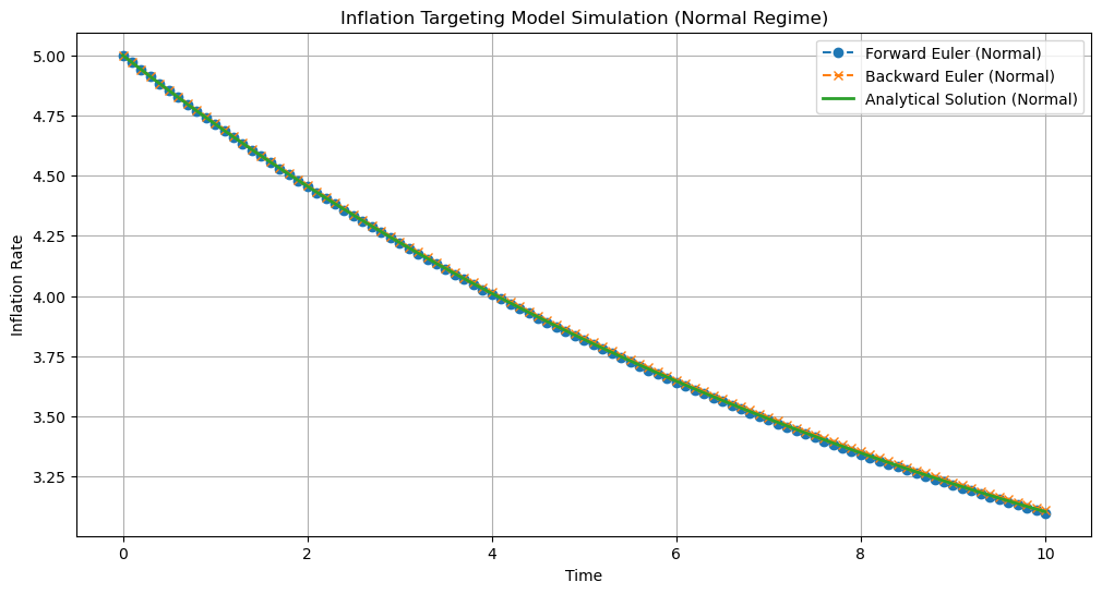
Fig. 7.1 Solution of the inflation targetting differential equation comparing the analytical solution with the forward and backward schemes. We choose a set of parameters and grid size where both methods approximate well the analytical solution: \(\theta = 0.1, \Delta = 0.1, \hat{\pi} = 2.0, \pi_0 = 5.0\)#
Let us now increase the grid size and choose another set of parameters to make the numerical approximation more challenging. We can see how the forward scheme deviates substantially from the analytical solution, whereas the backward scheme remains more robust:
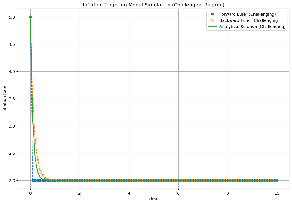
Fig. 7.2 Solution of the inflation targetting differential equation comparing the analytical solution with the forward and backward schemes. We choose a set of parameters and grid size where a numerical approximation is more challenging, to show the advantages of the backward scheme: \(\theta = 10, \Delta = 0.1, \hat{\pi} = 2.0, \pi_0 = 5.0\)#
7.3. The Wiener Process#
7.3.1. Definition#
So far we have discussed models where we neglect any uncertainty in the trajectories of the dynamical systems we are modelling. However, in many situations, randomness is a dominant characteristic of the process and we need tools to model such stochastic systems.
The Wiener process is the main building block when modelling stochastic dynamical systems which exhibit continuous trajectories. In order to model discrete jumps we will introduce later another building block, the Poisson process.
Many introductory books motivate the Wiener process as the continuous limit of a random walk, e.g. a discrete dynamical process in which each step is decided by a random binary variable \(Z_t = {1, -1}\) with \(p = 0.5\), i.e. analogous to flipping an unbiased coin. If we know that the process at time \(t\) is \(X_t\), then \(X_{t+1} = X_t + Z_t\).
Here, we will instead introduce the Wiener process as a fundamental building block for the modelization of stochastic processes, i.e. a tool that will allow us to capture certain observed or proposed behaviours of those systems in a model from which we can draw inferences. In such way, we define a Wiener process as a type of stochastic process, i.e. an (in principle infinite) sequence of random variables \(W_t\) indexed by time \(t\), with the following particular properties:
\(W_0 = 0\)
\(W_{t+s} - W_s \sim N(0, s)\) where \(N(0,s)\) is a Gaussian distribution with zero mean and variance \(s\), i.e. the increments of the Wiener process are Gaussian
\(W_t\) has independent increments, meaning that any \(W_{t_1}-W_{t_2}\), \(W_{t_3} - W_{t_4}\) where \(t_1 < t_2 < t_3 < t_4\) are independent
\(W_t\) has continuous trajectories
7.3.2. Connection to Gaussian Processes#
The specific properties of the Wiener process make it part of the family of Gaussian processes, which are stochastic processes with the property that any finite set of them, \(X_{t_1}, ..., X_{t_n}\) follow a joined multivariate Gaussian distribution. The Gaussian process can be described then by a mean function \(\mu_t = \mathbb{E}[X_t]\) and a covariance function \(k(t_1, t_2) = \textrm{cov}[X_{t_1}, X_{t_2}]\) that is usually referred as the kernel function of the Gaussian process.
The index for the stochastic process does not need to refer to time, another typical indexing is space, for instance. When using time as an index, we talk about Gaussian Processes for time-series modelling. This is the case for the Wiener process, which is a Gaussian process with mean \(\mu_t = 0\) and kernel:
In which sense it is useful to introduce this relationship? The theory of Gaussian processes has been pushed in the last years within the Machine Learning community, and there are multiple tools available for building, training and making inferences with these models. Such toolkit can be useful when building models for dynamical systems using stochastic processes.
7.3.3. Filtrations and the Martingale Property#
The Wiener process satisfies the Martingale property, meaning that if we have a series of observations of the process \(W_{t_1}, W_{t_2}, ... W_{t_n}\) then the expected value of an observation \(t_{n+1} > t_n > ... > t_1\) conditioned to the previous observations only depends on the last observation:
i.e., the information from previous observations is irrelevant. We can generalize the martingale property by introducing the notion of filtration \(F_t\) at time \(t\), which contains all the information set available until time \(t\). We can rewrite the Martingale property using the filtration as:
We can prove the Martingale property using the defining properties of the Wiener process:
where we have used that the increments of the Wiener process have zero mean.
7.3.4. The Tower Law#
A useful property that exploits the concept of filtration in many applications is the so-called Law of Iterated Expectations or Tower Law. It simply states that for any random variable Y, if \(t_m > t_n\):
This is a useful property to compute expectations using a divide and conquer philosophy: maybe the full expectation \(\mathbb{E}[Y|F_{t_n}]\) is not obviously tractable, but by conditioning it at intermediate filtrations \(\mathbb{E}[\mathbb{E}[\mathbb{E}[...\mathbb{E}[Y|F_{t_m}] ... |F_{t_{n+2}}|F_{t_{n+1}}|F_{t_n}]\) we can work out the solution. We will see examples later on.
7.3.5. Multivariate Wiener process#
We can construct a multivariate Wiener process as a vector \({\bf W}_t= (W_{1t}, W_{2t}, ..., W_{Nt})\) with the following properties:
\({\bf W}_t = {\bf 0}\)
\({\bf W}_{t+s} - {\bf W_t}_s \sim N(0, \Sigma s)\) where \(\Sigma\) is a NxN correlation matrix. This means that the increments of the components of the multivariate Wiener process might be correlated
\({\bf W}_t\) has independent increments, meaning that any \({\bf W}_{t_1}-{\bf W}_{t_2}\), \({\bf W}_{t_3} - {\bf W}_{t_4}\) where \(t_1 < t_2 < t_3 < t_4\) are independent
Each of the components of \({\bf W}_t\) has continuous trajectories
Ito’s Lemma We have seen that given the trajectory of a deterministic dynamical system, \(y_t = f(t, {X_t})\), its behavior over a infinitesimal time-step is described by the following differential equation:
where \(\{X_t\}\) is a set of deterministic external factors. But what if the external factors are Wiener processes, e.g. in the most simple case \(f(t,W_t)\)?. We might be tempted to just reuse the previous equation:
however, one of the peculiarities of the Wiener process is that this equation is incomplete, since there is an additional term at this order of the expansion. There are different ways to derive this result, typically starting from the discrete Wiener process (random walk), but a simple non-rigorous argument can be made by expanding the differential to second order in the Taylor series:
and take the expected value of this differential conditional to the filtration at t:
The key for the argument is that whereas \(\mathbb{E}[dW_t|F_t] = 0\), we have \(\mathbb{E}[dW_t^2|F_t] = dt\), getting:
so if we keep only terms at first order in the expansion:
we have an extra term coming from the variance of the Wiener process, whose expected value is linear in \(dt\). This motivates us to propose the following expression for the differential of a function of the Wiener process, the so-called Ito’s lemma:
The same argument can be applied for a multivariate Wiener process. Let us for example analyze the case of a function of two correlated Wiener processes, \(y = f(t, W_{1t}, W_{2t})\). Expanding to second order in a Taylor series we get:
Now, using the expected value argument and keeping only terms \(O(dt)\):
where we have used \(\mathbb{E}[d W_{1t} dW_{2t} |F_t] = \rho_{12} dt\) as discussed in the section on multivariate Wiener processes. This motivates the expression for the two-dimensional Ito’s lemma:
###Integrals of the Wiener process
A firs relevant integral of the Wiener process is:
What is the distribution of \(I_{1t}\)? A simple way to deduce it is to discretize the integral and then take again the continuous limit:
where \(\Delta = t / N\), \(u_i = \Delta i\). This is a sum of independent Gaussian random variables, since by definition the increments of the Wiener process are independent. Therefore its distribution is itself Gaussian [1]. Its mean is easily computed as:
For the variance, we could simply use the result that the variance of independent variables is the sum of variances, but it is instructive to compute it directly over the discrete expression:
The computation of \(\mathbb{E}[(W_{u_{i+1}} - W_{u_i})(W_{u_{j+1}} - W_{u_j})|F_0]\) needs to consider two cases. When \(i \neq j\) the expectation is zero, since increments of the Wiener process are independent. This is no longer the case of \(i = j\), for which we have \(\mathbb{E}[(W_{u_{i+1}} - W_{u_i})^2|F_0] = u_{i+1} - u_i = \Delta\). Therefore:
Plugging this into the previous equation:
Therefore, the distribution of \(I_{1t}\) is given by:
Notice that once we have motivated the solution by using a discretization of the equation, we can directly skip it and use the continuous version, for instance:
Let us now move into the second relevant integral of the Wiener process, namely:
What is the distribution of this random variable? In this case, applying the discretization argument does not provide a direct simple path to figure out the distribution, since we have a sum of correlated variables (e.g. \(f(W_{u_i})\) and \(f(W_{u_j})\) are correlated over the common paths shared by them, say if \(u_i < u_j\), the path below \(u_i\)). We can use Ito’s lemma to advance our comprehension:
which being linear it does not have the Ito’s convexity terms. Essentially we can then use integration by parts:
Using again Ito’s lemma, now on \(f(W_u)\):
we get:
At this point we cannot proceed further in general unless we specify specific functions. For instance, the most simple non trivial case is the linear function \(f(W_u) = W_u\). Applying this formulation:
which now we can identify as a specific case of the previous integral, with \(f(u) = t - u\). The distribution is therefore:
where we have used \(\int_0^t (t-u)^2 du = \frac{t^3}{3}\)
###Simulation of the Wiener process
We can simulate the Wiener process using a discretization like the Euler scheme for deterministic processes. Again, defining a grid \(t_i = t_0 + \Delta * i\), \(i = 0, .., N\), where \(\Delta = \frac{t_N - t_0}{N}\), we can exploit directly the Wiener process properties to get:
So we can simulate numerically the Wiener process simply as:
where \(Z\) is a standard normal distribution. The following plot simulates the Wiener process numerically for a few different paths:
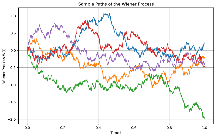
Fig. 7.3 Simulation of five different paths of the the Wiener process using \(t_0=0\) \(t_N=1\), \(N = 100\), \(W_0 = 0\)#
Alternatively, we can simulate complete paths of the Wiener process by exploiting its connection to Gaussian processes. Using a Gaussian process framework we get the following results:
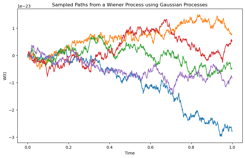
Fig. 7.4 Simulation of five different paths of the the Wiener process using the same parameters, but sampling from a Gaussian process with a Wiener \(min(t_1, t_2)\) kernel#
Multivariate processes
Let us now simulate a multivariate Wiener process of dimension N. The strategy in this case is to start simulating N independent Wiener processes and then use them to generate the correlated paths. This can be done using the Cholesky decomposition of the correlation matrix \(\Sigma\). Since \(\Sigma\) is symmetric and positive define, the decomposition reads:
where \(L\) is a lower triangular matrix. If we now we have a vector of N uncorrelated Wiener increments \(d \hat{{\bf W_t}}\), we can obtain the correlated process by using \(L\) such as \(d {\bf W_t} = L d \hat{{\bf W_t}}\). We can see that this vector has the distribution of the multivariate Wiener process increment:
where we have used \(\mathbb{E}[d \hat{{\bf W}}_{t} d \hat{{\bf W}}_{t}^T] = I dt\) where \(I\) is the identity matrix.
It is illustrative to show the case for a two-dimensional multivariate Wiener process. The correlation matrix reads:
The Cholesky lower triangular matrix is simply:
Notice that, as expected:
We can also write the decomposition in equations:
7.4. Stochastic differential equations#
As pointed out in the introduction to the chapter, after studying the Wiener process now we have the tools to model the dynamics of a random or stochastic process \(X_t\) using stochastic differential equations (SDEs) of the general form:
which generalizes the deterministic differential equation adding a noise term modelled using the Wiener process. Solving a SDEs means working out the distribution of \(X_t\) at arbitrary times given some initial conditions, which for arbitrary choices of \(\mu(X_t, t)\) and \(\sigma(X_t,t)\) can only be solved numerically, for instance using Monte-Carlo sampling techniques. In the next section we will see particular SDEs that are analytically tractable.
7.5. The Feynman - Kac Theorem#
The Feynman-Kac theorem provides a link between partial differential equations and stochastic processes, specifically, between certain types of PDEs and expectations of integrals of the Wiener process. Its usefulness extends to subjects like physics and finance, where it is used to introduce statistical interpretations of solutions to deterministic systems.
Specifically, the Feynman - Kac theorem it relates the solution \(u(x,t)\) of the PDE
with the boundary condition \(u(x,T) = f(x)\), to the expected value
where \(X_t\) satisfies the general SDE introduced in section {ref}` stochastic differential equation (SDE):
To prove it we use Ito’s lemma to compute the differential of the ansatz \(Y_s = e^{-\int_t^s r(X_v,v) dv} u(X_s, s)\):
which we can rewrite as $\(\begin{aligned} d Y_s = e^{-\int_t^s r(X_v,v) dv} \frac{\partial u}{\partial X_s} \sigma(X_s, s) dW_s + \\ e^{-\int_t^s r(X_v,v) dv} \left(-r(X_s, s) u + \frac{\partial u}{\partial s} + \frac{\partial u}{\partial X_s} \mu(X_s,s)+ \frac{1}{2} \frac{\partial ^2 u}{\partial X_s^2} \sigma^2(X_s,s) \right) ds = \\ e^{-\int_t^s r(X_v,v) dv} \frac{\partial u}{\partial X_s} \sigma(X_s, s) dW_s \end{aligned}\)$
where we have used that \(u\) is the solution to the above PDE to make the term in parenthesis zero. We can now integrate this equation from t to T:
If we take now expectations, the right hand term is zero by using the properties of the integral of the Wiener process show in previous sections. Therefore:
i.e. \(Y_t\) is a martingale. But this is actually the Feynman - Kac solution if we replace \(Y_t\) by its definition, since \(u(X_T, T) = f(X_T)\), which completes the proof.
7.6. Basic stochastic processes#
7.6.1. Brownian motion with drift#
The most simple stochastic process using the Wiener process as a building block is the Brownian motion with drift:
Here we are essentially shifting and rescaling the Wiener process to describe dynamical systems whose stochastic fluctuations have a deterministic non-zero mean \(mu_t\) (drift) and arbitrary variance, the latter controlled by the so-called volatility \(\sigma_t\). In practice, this is the process to use for any real application of stochastic calculus to model random time-series, since the simple Wiener process is simply too restrictive to describe any real process. The name Brownian motion comes actually from the early application of this kind of process to describe the random fluctuations of pollen suspended in water observed by English botanist Robert Brown in 1827. The actual modelling of this process would be pioneered by Albert Einstein [5], in one of the four papers published in 1905, his “annus mirabilis”, each of them transformative of its respective field.
The distribution of \(dS_t\) is easily derived by using the property that multiplying and summing scalars to a Gaussian random variable (\(dW_t\)) yields another Gaussian variable. Hence since \(dW_t \sim N(0, t)\) then we have:
This stochastic differential equation can be integrated to get the solution for arbitrary times:
which again follows a Gaussian distribution:
where we have used the properties of the stochastic integral discussed in section Stochastic differential equations:
Connection to Gaussian processes
The Brownian motion is also a Gaussian process, since any finite set \(S_{†_1}, S_{t_2}, S_{t_3}, ..., S_{t_n}\) follows a multivariate Gaussian process. The kernel of the Brownian process is simply to derive:
If \(\sigma_t = \sigma\), i.e. is a constant, we have simply:
which is the kernel of the Wiener process rescaled by \(\sigma^2\), as expected given the construction of the Brownian process.
To complete the specification we need to add a mean function, which is simply:
Simulation
Similarly to the Wiener process, simulation can be carried out using a discretization scheme. To improve numerical stability and convergence it is convenient to integrate first the distribution between points in the simulation grid \(t_0, ..., t_N\), \(t_{i+1} = t_i + \Delta t_i\), namely:
If we have a generator of standard Gaussian random numbers \(Z\), we can perform the simulation using:
If \(\mu_u\) and \(\sigma_u\) are smooth functions of time and \(\Delta t_i\) is small enough such that the variation in the interval is negligible, we can approximate the integrals:
or simply:
The following graph shows samples of the Brownian motion for specific values of drift and volatility:
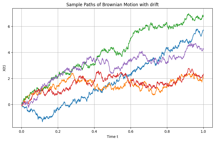
Fig. 7.5 Simulation of five different paths of the the Brownian Motion with drift process using \(t_0=0\) \(t_N=1\), \(N = 100\), \(W_0 = 0\), \(\mu = 5\), \(\sigma = 2\).#
Alternatively, we could use the connection to Gaussian processes to perform the simulations using standard packages. We leave it as an exercise for the reader.
Estimation
If we have a set of observations of a process \(D = \{S_{t_0}, ..., S_{t_N}\}\) that we want to model as a Brownian motion, we need to find the value of the parameters of the process that best fit the data.
Let us consider for simplicity that \(\mu_t = \mu\), \(\sigma_u = \sigma\) and \(\Delta t_i = \Delta t\) . As discussed in the context of Bayesian models, a general estimation process models the parameters as random variables that capture our uncertainty about their exact values, which comes from the fact that the sample is finite, or also in general because the data generation process will not necessarily be the one we are proposing, being models a simplification of reality. In this setup, the best inference of the parameters is carried out by computing the posterior distribution \(P(\mu, \sigma^2|D, I_P)\) where \(I_P\) represents the prior information about the parameters.
Since as shown in the previous section we can write the process between observations as \(S_{t_{i+1}} - S_{t_i} = \mu \Delta t + \sigma \sqrt{\Delta t_i} Z\) with \(Z\sim N(0,1)\), this is equivalent to fitting a Bayesian linear regression model om \(S_{t_{i+1}} - S_{t_i}\) with an intercept \(\mu \Delta t\) and a noise term \(\epsilon \sim N(0, \sigma^2 \Delta t)\). As we shown in chapter Introduction to Bayesian Modelling, if we model the prior distributions of the parameters as a Normal Inverse Gamma (NIG), meaning that:
where \(V_0\), \(\mu_0\), \(\alpha_0\), \(\beta_0\) are parameters that define the prior, this distribution is a conjugate prior of the likelihood:
Therefore, the posterior is also a NIG, with updated parameters:
To get the updated parameters from the general equations, bear in mind that in this representation with only an intercept our feature-set can be seen as a N dimensional vector \({\bf X} = (1, ..., 1)\). Therefore:
The predictive marginal for the \(\mu \Delta t\) parameter requires integrating out the \(\sigma^2 \Delta t\), resulting in:
where \(T\) is the Student’s distribution.
Following our discussion in chapter Introduction to Bayesian Modelling, the best estimator of parameters extracted from the posterior in a mean squared error minimizing sense is to compute the mean of the posterior marginals. For \(\sigma^2 \Delta t\), we have:
whereas for \(\mu\) we have:
A special case deserved our attention: if we take the limit in the prior distribution \(V_0\rightarrow\infty\) and \(\alpha_0, \beta_0 \rightarrow 0\), the prior distribution becomes a non-informative or Jeffrey’s prior, with \(p(\sigma^2 \Delta t) \sim 1/(\sigma^2 \Delta t)\), and \(p(\mu\Delta t|\sigma^2\Delta t)\) becoming a flat prior. Jeffrey’s prior is considered the best choice to describe non-informative priors of scale parameters as is the case of \(\sigma^2 \Delta t\). In this situation:
which are the maximum likelihood estimators (MLE) of the mean and the variance of a Gaussian distribution, which is expected for a non-informative prior since 1) for a Gaussian distribution the mean and the mode coincide, 2) maximizing the posterior with the non-informative prior is equivalent to maximizing the likelihood. MLE estimators are the standard approach to learn the parameters of stochastic processes in many practical situations, since the Bayesian estimations might become intractable for more complex processes as the Brownian motion. However, we must keep in mind their limitations, particularly that they neglect any prior information that might be useful in certain setups, and that they throw away the rest of the information contained in the posterior distribution.
We will see in later chapters that keeping the full posterior distribution can be relevant when we want to incorporate model estimation uncertainty into the inferences that are derived using stochastic processes. For instance, in the presence of a non-negligible estimation uncertainty of the parameters of our Brownian process, the correct predictive distribution of the next value of the process given its past history is actually given by:
If we consider a non-informative prior, this becomes:
This is to be compared with the inference using the MLE estimator, which would essentially plug the point MLE estimator into the Brownian process, yielding:
The mean and the mode of both distributions is the same, namely \(\mu_{MLE} \Delta t\), but the Student distribution has fatter tails than the Gaussian distribution, reflecting the extra uncertainty coming from the estimation error. Only in the case of having a very large data-set \(N\rightarrow \infty\), both distributions converge, as in this limit the Student distribution becomes a Gaussian \(N(\mu_{MLE} \Delta t, \sigma_{MLE} \Delta t)\). Another way of seeing this is to interpret the variance term of the Student distribution as the sum of two terms: the first one coming from the intrinsic noise of the Brownian process, and the second one, the \(1/N\) correction, coming from the estimation uncertainty.
Dimensional analysis
In order to reason about stochastic processes it is important to keep track or the units of their parameters. This can also be useful as a consistency check on the estimators derived, for instance. We will use a brackets notation for dimensional analysis. For the case of the Brownian motion we write:
In here, we know that \([dt]\) has time units, for instance seconds, hours, or days. We denote them generically as \([t]\) The Wiener process being distributed as \(dW_t \sim N(0, dt)\) has therefore units of \([t]^{1/2}\), i.e. the square root of time. Therefore, the parameters have the following units:
where we have denoted generically \([S]\) as the units of the process. If for instance \(S\) is modelling a price of a financial instrument in a given currency like dollars, the units are dollars: \([dS_t] = \$\). If additionally we are using seconds as time units, \([t] = s\). then we have \([\mu_t] = \$ / s\) and \([\sigma_t] = \$ / s^{1/2}\). We can see that these units are consistent with the Gaussian distribution for the evolution of \(S_t\): the argument of the exponential should be a-dimensional. Applying the previous units to the expression we can see that it is indeed the case:
Applications
The Brownian motion model has plenty of applications. In the financial domain it can be used to model financial or economical indicators for which there is no clear pattern in the time-series beyond potentially a drift to motivate a more sophisticated modelling, i.e. the time-series is mostly unpredictable. Notice that the Brownian motion has a domain that extends from \((-\infty, \infty)\), so indicators that have a more restrictive domain might not be suitable for being modelled using the Brownian motion process. A typical example are prices of financial instruments, which cannot on general grounds be negative. However, there might be exceptions to this rule, for instance if we are modelling prices in a time - domain such as the probability of reaching negative values is negligible, the model might be well suited. For instance, when modelling intra-day prices.
7.6.2. Geometric Brownian motion#
The geometric Brownian motion is a simple extension of the Brownian motion that introduces a constraint in the domain of the process, allowing only positive values. The stochastic differential equation is the following one:
In order to find the distribution of \(S_t\) for arbitrary times, let us apply Ito’s lemma over the function \(f(S_t) = \log S_t\). Such ansatz is motivated by looking at the deterministic part of the equation, \(dS_t = \mu_t S_t dt\), which can be rewritten as \(d \log S_t = \mu_t dt\). Coming back to the stochastic differential equation:
This is the stochastic differential equation of the Brownian motion, which we already now how to integrate from the previous section:
which means that \(\log S_t\) follows a Gaussian distribution
The distribution of \(S_t\) is the well studied Log-normal distribution, which by definition is the distribution of a random variable whose logarithm follows a Gaussian distribution:
We can also simply write:
An interesting property of the Log-normal distribution is the simple solution for its moments: $\(\begin{aligned} X \sim LN(\mu, \sigma^2) \nonumber \\ \mathbb{E}[X^n] = e^{n \mu + \frac{1}{2} n^2 \sigma^2} \end{aligned}\)$
In particular, the mean of the distribution is \(\mathbb{E}[X] = e^{\mu + \sigma^2/2}\) which we will use in multiple applications. This means, coming back to the Geometric Brownian Motion, that:
Connection to Gaussian processes
The Geometric Brownian Motion (GBM) is also closely related to Gaussian processes, as its logarithm follows a Brownian motion with drift. Therefore, any finite set \(\log(S_{t_1}), \log(S_{t_2}), \log(S_{t_3}), ..., \log(S_{t_n}) \) follows a multivariate Gaussian distribution.
The covariance kernel of the logarithmic process can be derived as:
which for constant volatility \(\sigma_u = \sigma\) simplifies to:
This is the same covariance kernel as that of a standard Brownian motion, but applied to the logarithm of the process, reflecting the Gaussian nature of the logarithmic returns of the GBM.
It only remains to add the mean process to the specification, which we have already calculated. Since we are working with the logarithm of the process, this is:
Simulation
We can again simulate the GBM either using a discretization scheme or the connection to Gaussian processes. When using the discretization scheme more robust results can attained by simulating a Wiener process and then using a discrete integration of the GBM:
where \(Z \sim N(0,1)\). We perform such simulation with constant parameters in the following figure:
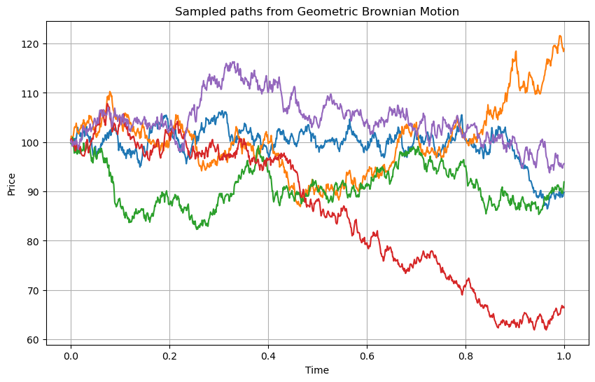
Fig. 7.6 Simulation of five different paths of the Geometric Brownian Motion with drift process using \(t_0=0\) \(t_N=1\), \(N = 1000\)\(, \)S_0 = 100\(, \)\mu = 0.05\(, \)\sigma = 0.2$.#
Estimation
The estimation of the Geometric Brownian Motion is relatively straightforward by linking it to a Brownian motion using log-returns. Therefore, we can transform a set of observations \(D = \{S_{t_0}, ..., S_{t_N}\}\) into \(D' = \{\log S_{t_0}, ..., \log S_{t_N}\}\) and apply any of the estimation techniques discussed in the previous sections.
Applications
The Geometric Brownian Motion is a corner-stone in financial modelling since it is the most simple model that captures non-negativity of asset prices like stocks. Therefore it has been applied in multiple context. For example, it was the model used by Black, Merton and Scholes for their infamous option pricing theory. It is also used typically in risk management use cases to simulate paths to compute value at risk (VaR).
7.6.3. Arithmetic mean of the Brownian motion#
As the name suggests, this is a derived process from the standard Brownian motion in which the latter is averaged continuously from a certain initial time to \(t\). We take for simplicity the initial time \(t_0 = 0\):
To derive its distribution we integrate by parts the Brownian process:
In this form, it is easy to derive the distribution, which is normal. Assuming for simplicity constant mean and volatility:
Notice that the variance of the average process is smaller than the variance of the process itself, by a factor \(1/3\). This makes sense, since taking averages smooths out the random behavior of the process.
Connection to Gaussian Processes
The arithmetic mean of Brownian motion is closely connected to Gaussian processes. Since the underlying process, \(S_t\), is itself a Gaussian process, the arithmetic mean \(M_t\), being a linear transformation of the Brownian motion, also follows a Gaussian process.
For any finite set of times \( M_{t_1}, M_{t_2}, \dots, M_{t_n} \), the joint distribution of these variables is multivariate Gaussian. To derive the covariance, let us first consider the zero-mean process:
where have simply used the definition of the process and used \(dS_u = \mu du + \sigma dW_u\). The covariance structure of the arithmetic zero-mean process can be derived as follows:
When \(t_1 < t_2\) we have:
Symmetrically, when \(t_1 > t_2\):
Therefore:
As in the previous processes, if we are starting from a non-zero mean and / or the Brownian motion has drift, we need to add the mean:
Simulation
Simulating the arithmetic mean does not present any extra complication with respect to the Brownian motion. We can discretize the underlying Brownian motion and simulate it, computing the mean at every step using the previous simulated values, i.e.:
Alternatively, we can use the kernel function derived above and generate paths of the Gaussian process. The following example uses GPs:
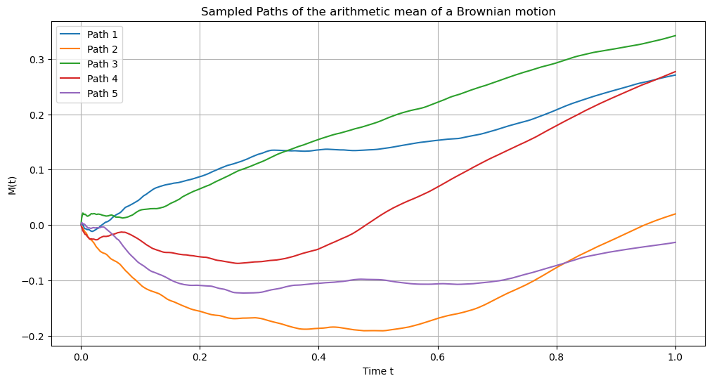
Fig. 7.7 Simulation of five different paths of the arithmetic mean of the Geometric Brownian Motion with drift process using the correspondence to Gaussian Processes. Parameters: \(t_0=0\) \(t_N=1\), \(N = 1000\)\(, \)S_0 = 0\(, \)\mu = 0.5\(, \)\sigma = 0.3$.#
As expected, the paths from the arithmetic mean are smoother than the ones from the underlying process, since they are averaged.
Estimation
Given a dataset of observations of the mean, \(D = \{M_{t_1}, ..., M_{t_N}\}\), the question is how to estimate the parameters of the underlying Brownian motion with drift. A priori, since the means are correlated, this could be a potentially complicated task. However, if we make the following transformation of the dataset:
these new variables are independent. We can therefore use standard Maximum Likelihood Estimators for the mean and variance of independent Gaussian random variables to obtain \(\mu\) and \(\sigma\).
Applications
In the financial modelling domain, arithmetic means of stochastic processes are used for instance when modelling so-called Asian options, whose underlying is precisely the arithmetic mean of the price of a financial instrument. For Asian options on stocks, which is the typical case, a Geometric Brownian Motion (GBM) is used to model prices to ensure non-negativity, and therefore rigorously speaking is the arithmetic mean of the GBM the underlying.
7.6.4. Orstein-Uhlenbeck process#
The Orstein - Uhlenbeck process is an extension of the Brownian motion process in which the drift term is modified to prevent large deviations from the mean \(\mu\). This is achieved by making the drift penalize those deviations:
The strength of the penalty is controlled by a parameter \(\theta > 0\), which is called the mean reversion speed: the larger this parameter, the faster the process \(S_t\) reverts to the mean. Such property of mean reversion is not unique to the Orstein - Uhlenbeck process, but the latter is probably the most simple way to achieve this effect in a stochastic differential equation, allowing for the computation of closed-form solutions for the probability distribution of the process. To derive it, we use the following ansatz:
Integrating this equation:
Finally:
Therefore, the Orstein - Uhlenbeck process follows a Gaussian distribution with time dependent drifts and variances:
The process has a natural time-scale, the mean reversion time, \(\tau \equiv 1/\theta\). For times \(t \gg \tau\) the distribution becomes stationary around the long-term mean:
The variance of the stationary distribution is no longer time - dependent, as in the Brownian motion process. Due to the pull-back effect that the mean reversion induces in the process around the long-term mean, the process remains bounded and stable over time.
Connection to Gaussian Processes
Given the previous analysis on the distribution of the Orstein - Uhlenbeck process, which is Gaussian, we can readily see that for any finite set of times, the joint distribution of \( S_{t_1}, S_{t_2}, \dots, S_{t_n} \), is multivariate Gaussian. The Orstein - Uhlenbeck is therefore a Gaussian Process with kernel given by:
where we have used that \(t_1 + t_2 - 2 \min(t_1, t_2) = |t_1 - t_2|\) to simplify the expression.
The specification so far only describes the mean-reverting fluctuations around the long-term mean. To complete the mapping to a Gaussian process of the full Orstein - Uhlenbeck process we need to add the mean to the specification:
Simulation
The simulation of the Orstein - Uhlenbeck process can be done once again by using a Euler discretization scheme of the SDE or exploiting the connection to Gaussian processes. If we use the former, it is convenient as it happened with the Geometric Brownian Motion, not to work directly with a discretized SDE, but to solve the equation for the discrete time step and sample from the Gaussian distribution:
The following picture shows such simulation. The initial condition is far from the long-term mean, showing a clear reversion until the stationary state is reached, over a time-scale proportional to the inverse of the mean-reversion speed \(\theta\).
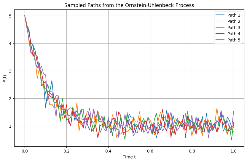
Fig. 7.8 Simulation of five different paths of the Orstein Uhlenbeck process using \(t_0=0\) \(t_N=1\), \(N = 1000\)\(, \)S_0 = 5\(, \)\mu = 1\(, \)\theta = 10\(, \)\sigma = 1$.#
Estimation
Given a set of observations \(D = \{ S_{t_i}, ..., S_{t_N}\}\), we can use maximum likelihood estimation to find the parameters of the model. The The log-likelihood function \(\mathcal{L}\) for the observed data is:
where:
Due to the complexity of the log-likelihood function, finding closed-form solutions for all the parameters is not possible, and we need to resort to numerical optimization.
However, under the assumption of equally spaced observations \(\Delta t_i = \Delta t\), we can simplify the estimation process linking the model to a linear regression problem. Define:
The process can be written in discrete time as:
where \(\varepsilon_i \sim \mathcal{N}(0, \psi^2) \). We can estimate \(\phi\) and \(\mu\) by regressing \(S_i\) on \(S_{i-1}\):
where \(\beta_0 = \mu \gamma\) and \(\beta_1 = \phi\). The ordinary least squares (OLS) estimation yields:
which is the first-order auto-correlation function. Moreover:
where the last approximation holds for a large enough number of samples. We can now come back to the original parameters. Starting with the long-term mean, Since \(\beta_0 = \mu \gamma = \mu (1 - \phi)\) and \(\phi = \beta_1\):
The mean-reversion speed reads
Finally, to estimate the variance, we use the definition of \( \psi^2 \):
Therefore, the estimator is:
where \(\psi^2\) is the residual variance of the regression, which is estimated as: $\( \hat{\psi}^2 = \frac{1}{n} \sum_{i=1}^n (S_{t_i} - \hat{\beta}_0 - \hat{\beta}_1 S_{t_{i-1}})^2 \)$
Applications
The Orstein - Uhlenbeck process can be applied to a variety of real phenomena. In the financial and economical domain, we find mean reversion in multiple processes like:
Inflation: which is influenced by central bank policy with specific inflation targets. For example, 2% in the Eurozone.
Interest rates: also influenced by central bank policy, as a way to affect inflation. It is also monitored by governments in order to ensure individual and companies can borrow money in competitive conditions.
Commodity prices: subject to supply and demand forces, stationality and, in some cases like oil, explicit intervention by organizations like OPEC, which use their oligopolistic control of supply to ensure prices remain within a range that is not too low to affect profits and too high to incentivise the switch to alternative sources.
Statistical arbitrage: prices of financial instruments might not show mean reversion, but combinations of them sometimes do. For example, pairs of stocks of companies with similar fundamentals.
Other mean reverting processes
Despite the popularity of the Orstein - Uhlenbeck process to model mean - reverting processes due to its simplicity and tractability, it has limitations in the type of models that can describe. For instance, for processes that can only take positive values, and the mean reversion time is independent of the distance to the long-term mean.
A popular related model is the Cox-Ingersoll-Ross (CIR) process, which is a variation of the Orstein-Uhlenbeck process, but with the added feature that the volatility term depends on the square root of the process itself, ensuring that the process remains positive.
The CIR process is given by:
Again, \(\theta > 0\) controls the speed of mean reversion, \(\mu\) represents the long-term mean level, and \(\sigma\) is the volatility. Unlike the Orstein-Uhlenbeck process, where the volatility is constant, the CIR model introduces a state-dependent volatility term \(\sqrt{S_t}\), which ensures that \(S_t\) stays positive (as the volatility goes to zero when \(S_t\) approaches zero). As a byproduct, the mean reversion time also depends on the actual value of the process.
Though no closed-form solution exists for the CIR process as simple as the one for the Orstein-Uhlenbeck process, it is often analyzed through numerical methods or approximations. The Fokker-Planck equation corresponding to the CIR process can be solved to obtain the transition probability density, which follows a non-central chi-squared distribution.
The CIR process is widely used in financial applications, such as in the modeling of short-term interest rates and in the Heston model for stochastic volatility, due to its ability to capture mean reversion and maintain non-negativity.
Other alternatives to the Orstein - Uhlenbeck process that allow to specifically model the behaviour of the mean reversion time are non linear drift models in the form:
where \(f(\cdot)\) is function of the distance to the mean, for instance a power law.
7.6.5. Brownian bridge#
Another simple extension of the Wiener process is the Brownian bridge, that we denote as \(B_t\). It defines a stochastic process within a time interval \([0,T]\) that behaves as a Wiener process with the exception of having an extra constraint, namely that \(B_T = 0\) (in addition to \(B_0 = 0\) as in the Wiener process). Such process can be constructed from a single Wiener process \(W_t\) as follows:
In order to derive the distribution of \(B_t\), we decompose it in two independent Gaussian variables:
where the two terms of the expression are independent by using the property that non overlapping differences of Wiener processes are independent. This is therefore the distribution of two independent Gaussian variables, which we know is also Gaussian:
where we have used:
The result fits well our expectation of such process: for \(t = 0\) and \(t = T\), the process has no variance, since those points correspond to the constraints where the process is set to zero. Given those constraints, and the symmetry of the Brownian bridge with respect to the transformation \(t \rightarrow T-t\), we expect the maximum variance to be at the half-point \(T/2\), which is indeed the maximum of the function \(t(1-\frac{t}{T})\)
Connection to Gaussian processes
The Brownian bridge is also a Gaussian process, with the following kernel:
The kernel has two terms: the first one corresponds to the kernel of a Wiener process, whereas the second one is a correction that reflects the boundary conditions of the Brownian bridge, i.e. the increasing certainty as we approach \(t \rightarrow T\). Mathematically, we have \(k(0,0) = 0\) as in the Brownian motions, but the additional constraint \(k(T, T) = 0\), specific from the Brownian motion.
Simulation
As usual, we can simulate the process either discretizing the stochastic differential equations or exploiting the Gaussian processes connection. If we want to approach the problem using discretization, the most simple way to do it is to simulate a discrete Wiener process which is then plugged into the Brownian Bridge expression.
In the following picture we follow the other path and simulate the Brownian Bridge using Gaussian Processes:
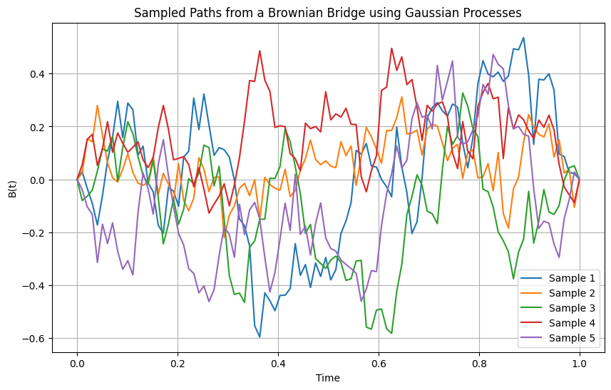
Fig. 7.9 Simulation of five different paths of the the Brownian Bridge using \(t_0=0\) \(t_N=1\), \(N = 100\).#
Applications
Brownian bridges or more realistic but similarly constructed processes (e.g. using the Brownian motion as the primitive instead of the Wiener process, or specifying fixed but non-zero boundaries), can be used to model situations where there is no uncertainty about the final value of a stochastic process. This is for instance the case of financial instruments like bonds, in particular zero-coupon bonds, which are bonds that simply return their principal at maturity without paying a coupon.
7.7. Jump processes#
So far we have described a family of continuous stochastic processes, with the Wiener process as the primitive to model different behaviors that can be useful to describe multiple phenomena. However, in many real situations we observe discrete jumps that are not rigorously described by these stochastic models, for which the probability of a jump of any size tends to zero as \(dt \rightarrow 0\).
Of course, one could argue that a continuous model is in general wrong in many applications, and it is only used in practice because of tha mathematical tractability. Take for instance price series of financial instruments. At some time-scale determined by the infrastructure of the exchange, prices simply move discretely tick by tick, and a continuous model is no longer a good description of the times-series at this time-scale.
As mentioned, though, continuous models are in fact a good description of financial price-series at time-scales of interests for many trading models, continuity being a natural reflection of investors taking the last price traded as the reference for successive valuations. However, even in those time-scales we observe sometimes price movements in a short period of a magnitude that a continuous model cannot account for. Examples are for example 2010’s flash-crash in the US market when using a time resolution of minutes, or October 1989’s Black Friday when using end of day prices.
This is not because the distributions derived in the continuous stochastic processes studied so far don’t allow those scenarios. Think for instance that the Gaussian distribution has non-zero probability density over the entire domain, and in real applications one could argue that the jump does not happen instantaneously if short enough time-scales are observed. But they are so unlikely under the model that any real application built upon them will not take into account those scenarios in practice, introducing potential risks. In other words, they are not good generative models of the phenomenon at hand, since such scenarios will not in practice expected when sampling or simulating from them.
Given that we still want to exploit the mathematical simplicity of continuous stochastic processes, we would like to introduce mathematical tools that allow us to incorporate discrete jumps with a meaningful probability in these models. The motivation is again that of mathematical simplicity, since one could argue that more complex continuous models could be built to describe those situations, as far as we agree that at a short enough time - scale what we observe as a jump can be described as a rapidly series of continuous changes. For instance, a model with regime switches in volatility. However, such complexity would penalize the applications of the model, hence the interest in modelling jumps in continuous time.
In the following section we will motivate such model, that we will formalize later on.
7.7.1. Poisson processes#
Motivation: a simple model for jumps in continuous time
We want to develop a model that allows for jumps of a given size \(J\) to happen instantaneously in continuous time. We denote by \(N_t\)the number of jumps that have accumulated in the time interval \([0, t]\). We make the hypothesis that a jump between time \(t\) and \(t + dt\) happens with a probability that is independent of the number of jumps so far:
where \(\lambda\) is a constant. This means, on the other hand, that:
since we are keeping terms up to \(O(dt)\).
Applying the rules of probability, we can express the probability of having \(n\) jumps up to time \(t + dt\) as:
Reorganizing the equation we get:
Taking the limit as \(dt \rightarrow 0\), this becomes a differential equation:
For \(n = 0\), this equation simplifies to:
whose solution is, with the initial condition \(P(N_0 = 0) = 1\):
which is called the first jump probability. For \(n = 1\) we have:
We can rewrite the equation as:
Therefore the solution that satisfies the initial condition is \(P(N_t = 1) = e^{\lambda t} \lambda t\). Continuing with \(n = 2\) we have the differential equation:
which can be again rewritten as:
And the solution is now \(P(N_t = 2) = \frac{(\lambda t)^2}{2} e^{-\lambda t}\).
At this point a patterns starts to be clear in the recursive solution as to apply the inductive step and propose a solution of the following form that generalizes the previous solutions:
Which we can see that satisfies the recursive differential equation:
We recognize this expression as the Poisson distribution function with an intensity \(\lambda\). Therefore this is called a homogeneous Poisson process, in contrast to non-homogeneous Poisson processes where the intensity is a deterministic function of time \(\lambda_t\).
The previous demonstration can be easily reproduced in this case. The differential equation reads now:
with the following solution, that can also be constructed inductively:
There are other two related processes that is worth to mention: we have a self-exciting or Hawkes process when the intensity is a function of previous number of jumps, namely:
where \(\mu_t\) is a deterministic function (the background intensity). \(\tau_i\) is the time at which jump \(i\) happened, and \(\nu\) is the excitation function, a deterministic function that controls the clustering of jumps. A popular choice is an exponential shape: \(\mu(t - \tau_i) = \alpha e^{-\beta(t- \tau_i)}\).
Finally, if the intensity is itself a stochastic process, we have a Cox process.
Definition and general properties
A counting process \(N_t\) is called a Poisson process with rate \(\lambda > 0\) if it satisfies the following properties:
\(N_0 = 0\): the process starts with zero events at time zero.
Independent increments: The numbers of events occurring in disjoint time intervals are independent. That is, for any \( 0 \leq s < t \), the number of events in \([s, t]\) is independent of the events before time \(s\).
Stationary increments: The probability distribution of the number of events occurring in any time interval depends only on the length of the interval, not on its position on the time axis. Specifically, for a homogeneous Poisson process, the number of events in an interval of length \(t\) follows a Poisson distribution with parameter \(\lambda\):
\[ P(N_{t + s} - N_s = n) = \frac{(\lambda t)^n}{n!} e^{-\lambda t} \]No simultaneous events: The probability of more than one event occurring in an infinitesimally small interval \(dt\) is negligible, specifically of order \(O(dt)\).
An important property of the Poisson process is that the times between consecutive events, known as inter-arrival times, are independently and identically distributed (i.i.d.) exponential random variables with parameter \(\lambda\):
where \(T_i\) is the time between the (i-1)-th and the i-th event, a random variable with probability density:
The derivation of this property is straightforward since we can link both distributions:
The exponential distribution of inter-arrival times implies the memory-less property: the probability that an event occurs in the next \(t\) units of time is independent of how much time has already elapsed since the last event. The average inter-arrival time is easy to compute as:
Mean and variance:
For a Poisson process with rate \(\lambda\), both the expected value and the variance of \(N_t\) are linear in time:
This reflects that the mean number of events grows linearly with time, and the variance equals the mean.
Estimation
The estimation of Poisson processes is relatively straightforward since they are characterized by a single parameter \(\lambda\), which is directly linked with the mean of the process \(E[N_t] = \lambda t\). Therefore, by computing the average number of jumps in a given time interval we can quickly estimate this parameter.
Simulation
Simulating Poisson processes is relatively simple by discretizing time in a grid with time-step \(\Delta t\). Then we can approximate:
which is a random binary variable with probability \(\Delta t\). Therefore, starting at \(t = 0\), we can build paths of the Poisson process by using samples of this binary variable. At every time-step \(t_i\) we keep or increase the counter \(N_{t_i}\) depending on the result. The following plot shows such simulation of a Poisson process.
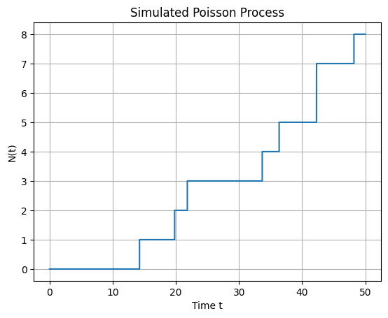
Fig. 7.10 Simulation of a Poisson process in a discrete grid with 50 time-steps and intensity \(\lambda = 0.2\)#
The same method can be used for more complex jump processes. For example, the following plot has been generated for a Hawkes process using a exponential excitation function. In this case, jumps tend to cluster together in comparison with the behaviour of the Poisson process.
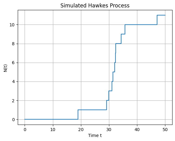
Fig. 7.11 Simulation of a Hawkes process in a discrete grid with 50 time-steps. The baseline intensity is again \(\lambda = 0.2\). The excitation function is an exponential with \(\alpha = 0.5\) and \(\beta = 1\).#
Applications:
Poisson processes are widely used to model random events in various fields, like queueing theory or telecommunications. In finance, they are typically used to model the arrival of orders (RfQs, limit or market orders), or to simulate defaults of companies, in which case only a single jump is allowed (jump to default).
They can also model jumps in financial prices, for instance in end of day time series, that incorporate the effect of unexpected news. For this application, though, these processes need to be generalized to incorporate random jumps (compound Poisson processes) and be included in Brownian price diffusions that model the evolution of prices in normal situations (jump diffusion processes).
7.7.2. Compound Poisson processes#
In many applications, events not only occur randomly over time but also have random magnitudes or impacts. A compound Poisson process extends the Poisson process by allowing for random jump sizes.
A compound Poisson process \(X_t\) is defined as:
where:
\(N_t\) is a Poisson process with rate \(\lambda\).
\(\{ Y_i \}\) are i.i.d. random variables representing the sizes of the jumps occurring at event times.
The \(Y_i\) are independent of the Poisson process \(N_t\).
Compound Poisson processes have the following properties:
Independent increments: The increments \(X_{t + s} - X_s\) over non-overlapping intervals are independent.
Stationary increments: For a homogeneous Poisson process, the statistical properties of increments depend only on the length of the interval, not its position.
Distribution of \(X_t\): The distribution of \(X_t\) is determined by both the distribution of \(N_t\) and the distribution of the jump sizes \(Y_i\).
Mean and variance:
The mean and variance of a compound Poisson process can be calculated using Wald’s equation, which states that the mean of the sum of real-valued, independent and identically distributed random variables \(x_i\), of which there are a random number of them \(N \geq 0\), is:
This result can be proven simply by conditioning the expected value on \(N\):
where we have used that \(\mathbb{E}[x_1]\) is independent of \(N\). Coming back to the definition of compound Poisson process:
A similar reasoning can be applied to the variance:
Simulation:
To simulate a compound Poisson process we simulate first the number of events \(N_t\) occurring up to time \(t\) using a Poisson distribution with parameter \(\lambda t\). Then, for each event \(i = 1, \dots, N_t\), we sample a jump size \(Y_i\) from the specified distribution. Finally, we sum the jump sizes to obtain \(J_t = \sum_{i=1}^{N_t} Y_i\).
A result of such simulation is shown in the following figure, with jumps being driven by an exponential model.
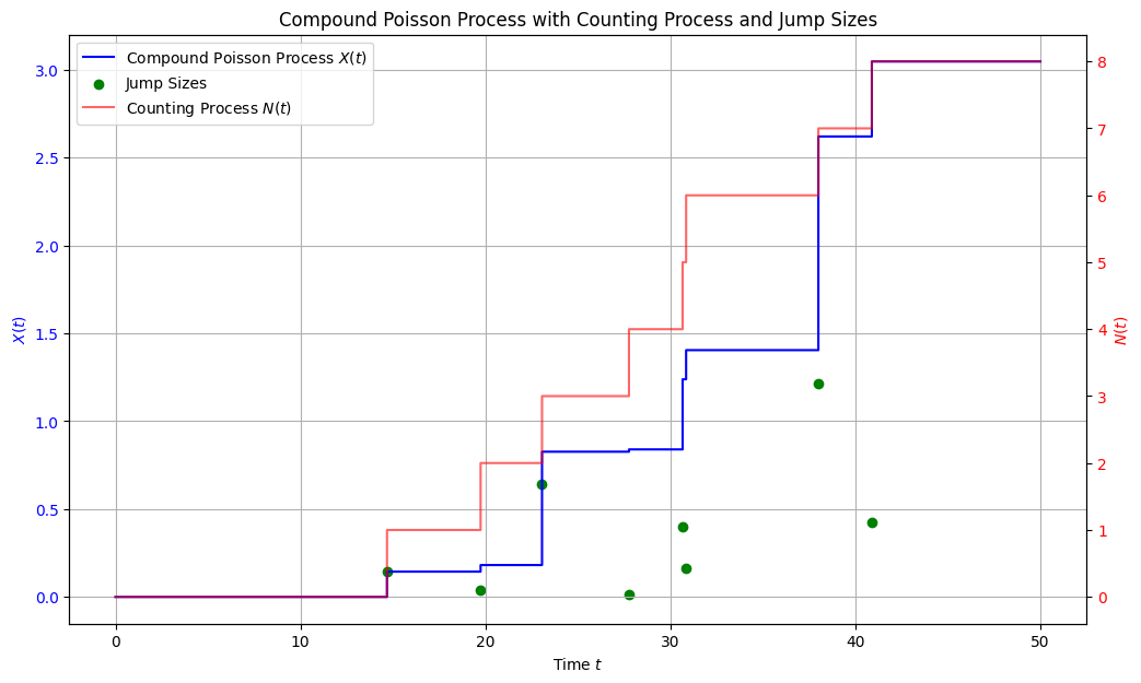
Fig. 7.12 Simulation of a compound Poisson process in a discrete grid with 50 time-steps. The baseline intensity is \(\lambda = 0.2\). For the distribution of jumps we use a exponential distribution with rate \(\eta = 2.5\). We plot separately the underlying Poisson process result and the simulated jump sizes, as well as the resulting compound process.#
7.7.3. Jump Diffusion Processes#
So far we have discussed jump processes that simulate discrete random events. But we would like to combine them with the continuous stochastic processes we studied in the previous part of this chapter, in order to generate richer dynamics to model real phenomena.
A jump diffusion process \(X_t\) is a stochastic process that combines a standard diffusion process with a jump component. It can be defined by the stochastic differential equation (SDE):
where:
\(\mu(X_{t^-}, t)\) is the drift coefficient, representing the deterministic trend.
\(\sigma(X_{t^-}, t)\) is the diffusion coefficient, representing the volatility.
\(W_t\) is a Wiener process
\(J_t\) represents the jump component, with \(J_t\) a compound Poisson process \(J_t = \sum_{i=1}^{N_t} Y_i\)
\(X_{t^-}\) denotes the value of \(X_t\) just before time \(t\), accounting for any discontinuities at \(t\).
As with the Wiener process, the differential of the jump process is a shorthand notation for \(dJ_t = J_{t+dt} - J_t\), i.e. the number of jumps happening between \(t\) and \(t+dt\). As we saw above, in a compound Poisson process since the intensity is \(\lambda dt\) only one or zero jumps are possible in the limit \(dt \rightarrow 0\). Therefore, we can simply write:
with \(P(dN_t = 1) = \lambda dt\).
Ito’s Lemma with Jumps
To analyze functions of jump diffusion processes, we need to extend the classical Ito’s lemma to account for jumps. The Ito’s lemma with jumps provides a framework for calculating the differential of a function applied to a process that includes both continuous and jump components.
Let \(X_t\) be a jump diffusion process defined above, and let \(f(X_t, t)\) be a twice continuously differentiable function in \(x\) and once differentiable in \(t\). Then, the differential \(df(X_t, t)\) is given by:
where \(\Delta X_t = X_t - X_{t^-} = Y\) is the jump size at time \(t\).
As we argued in the case of a Wiener process, the derivation can be motivated using a Taylor series expansion on the function for the continuous part, only adding the jump process, which is orthogonal to the continuous stochastic dynamics. When adding the jump component, the function \(f(X_t,t)\) changes discretely, hence the term \(f(X_{t^-} + \Delta X_t, t) - f(X_{t^-}, t)\) instead of the derivative. We only keep in this case the expansion up to \(dN_t\) since \(\mathbb{E}[dN_t] = \lambda dt\) which is already of order \(O(dN_t)\), so any extra term in the expansion will have a higher order.
Example: Merton’s jump diffusion model One of the main applications of jump diffusion models in the financial context is to model jumps in financial instruments that otherwise diffuse continuously.
One famous instance of such models incorporating jumps is Merton’s jump diffusion model [6], which model the dynamics of the asset with a Geometric Brownian Motion with jumps in the returns. The SDE for the asset price \(S_t\) is:
where \(\mu\) is the expected return rate, \(\sigma\) is the volatility, \(Y\) is a random variable representing the jump multiplier, and \(dN_t\) indicates the occurrence of a jump, modeled by a Poisson process with intensity \(\lambda\).
A typical choice to model jumps in this setup is using a log-normal distribution for the jumps, \(\log Y \sim \mathcal{N}(k, \delta^2)\)
In order to derive the distribution that follows this process, we can apply Ito’s lemma with jumps to the logarithm of the process, \(f(S_t) = \log S_t\), as we did analogously with the Geometric Brownian Motion, to which this model reduces in the absence of jumps. Since we have:
Then:
Therefore, the logarithm of the process follows a more simple dynamics composed of a Brownian motion with drift plus a jump that does not depend on the magnitude of the process. For Merton, this was a convenient way of introducing jumps in the returns of a financial instrument.
Simulation
Simulating jump diffusion models is relatively simple given what we have learnt so far, since we can proceed step by step by simulating independently the deterministic, the continuous stochastic and the jump components. The following simulation of the Merton model has been generated using such method.
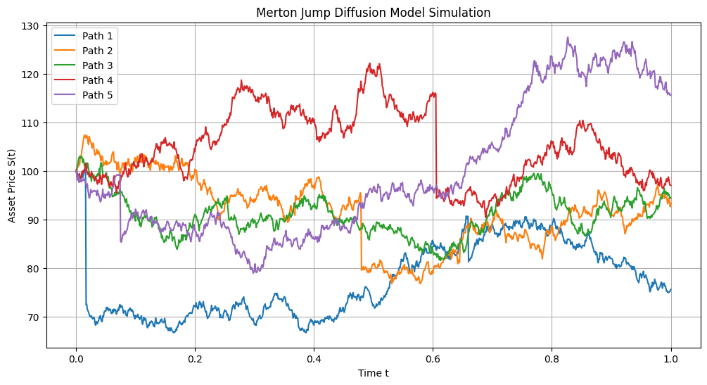
Fig. 7.13 Simulation of five paths of a jump diffusion process in a discrete grid with 1000 time-steps. The baseline intensity is \(\lambda = 1\). The Geometric Brownian Motion has drift \(\mu = 0.1\) and volatility \(\sigma = 0.2\) For the distribution of jumps we use a log-normal distribution with mean \(k = -0.1\) and standard deviation \(\delta = 0.1\).#
Applications
We have already mentioned the application of these models to simulating price series with jumps that might happen due to unexpected news or other disruptions in markets like sudden drops of liquidity. These models can be used to improve pricing and risk management of derivatives, or optimal market-making models. We discussed above that another typical application is modeling the jump to default of a corporation or government. Jump diffusion models are then used to model the impact in traded instruments influenced by credit risk, like bonds issued by those entities or credit default swaps linked to them.
For more theory or applications of jump diffusion processes, a good reference is that or Cont & Tankov [7].
7.8. Exercises#
Derive the Crank - Nikolson scheme discretization of the inflation targeting model. Simulate it numerically and compare with the exact solution
Use Ito’s lemma to derive the differential of:
\(f(W_t) = W_t^2\)
\(f(W_t) = t W_t\)
\(f(W_t) = \exp(W_t)\)
Simulate a Brownian motion with drift using the connection to Gaussian Processes.
Find the solution to the recursive differential equation: $\(\frac{d}{dt} P(N_t = n) = -\lambda P(N_t = n) + \lambda P(N_t = n - 1)\)$ using the method of the generating function, which we introduce as:
\[G(t,s) \equiv \sum_{n=0}^{\infty} P(N_t=n) s^n\]Hint: multiply the differential equation by \(s^n\) and sum over \(n\) to rewrite it as a function of the generating function. Solve the equation and express the solution as a Taylor series, matching the coefficients with \(P(N_t =n)\)