Stochastic Calculus

Deterministic dynamical systems

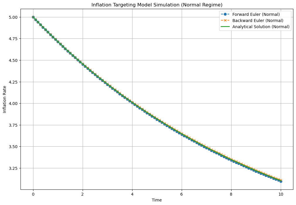
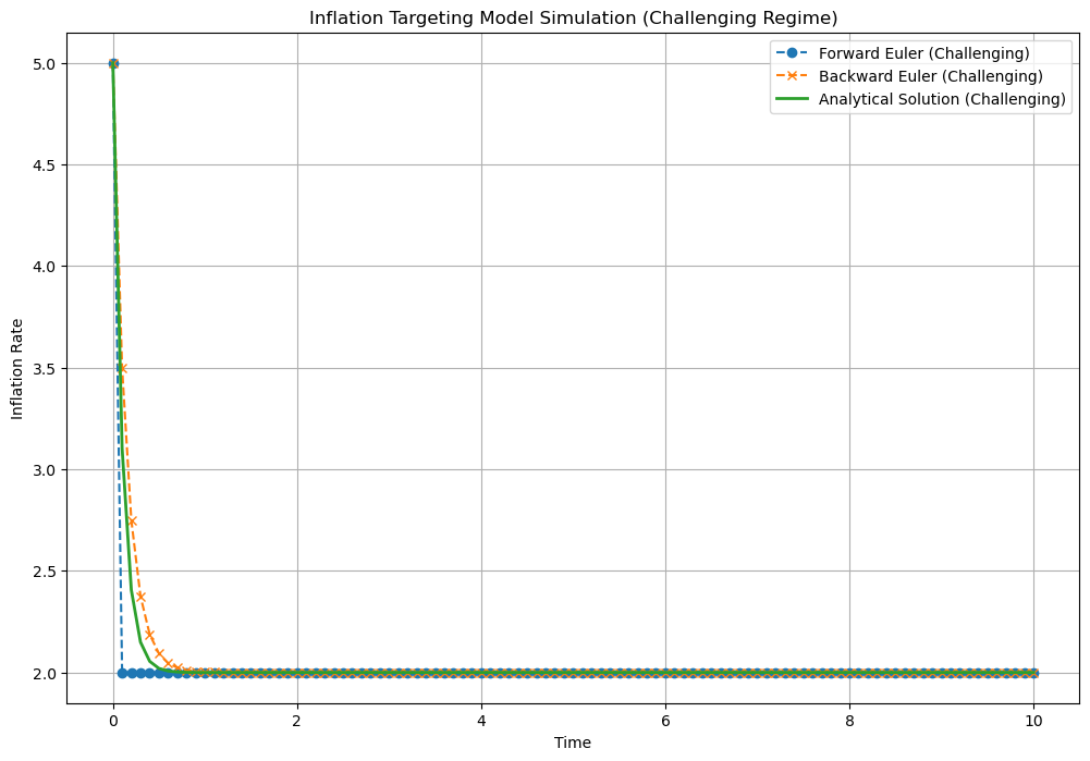
Numerical solution of dynamical systems: inflation targetting

import numpy as np
import matplotlib.pyplot as plt

def simulate_inflation(theta, pi_hat, pi_t0, Delta, N):
    # Time grid
    time = np.linspace(0, N * Delta, N + 1)

    # Arrays to store the results
    pi_forward = np.zeros(N + 1)
    pi_backward = np.zeros(N + 1)
    pi_analytical = np.zeros(N + 1)

    # Initial condition
    pi_forward[0] = pi_t0
    pi_backward[0] = pi_t0

    # Analytical Solution
    pi_analytical = pi_hat + (pi_t0 - pi_hat) * np.exp(-theta * time)

    # Forward Euler Scheme
    for i in range(N):
        pi_forward[i + 1] = pi_forward[i] + Delta * theta * (pi_hat - pi_forward[i])

    # Backward Euler Scheme
    for i in range(N):
        pi_backward[i + 1] = (pi_backward[i] + Delta * theta * pi_hat) / (1 + Delta * theta)

    return time, pi_forward, pi_backward, pi_analytical

# Parameters for normal regime
theta_normal = 0.1
Delta_normal = 0.1
pi_hat = 2.0
pi_t0 = 5.0
N = 100

# Parameters for challenging regime
theta_challenging = 10.0
Delta_challenging = 0.1

# Simulate for normal regime
time_normal, pi_forward_normal, pi_backward_normal, pi_analytical_normal = simulate_inflation(
    theta_normal, pi_hat, pi_t0, Delta_normal, N)

# Simulate for challenging regime
time_challenging, pi_forward_challenging, pi_backward_challenging, pi_analytical_challenging = simulate_inflation(
    theta_challenging, pi_hat, pi_t0, Delta_challenging, N)

# Plot the results for normal regime
plt.figure(figsize=(12, 8))
plt.plot(time_normal, pi_forward_normal, label='Forward Euler (Normal)', marker='o', linestyle='--')
plt.plot(time_normal, pi_backward_normal, label='Backward Euler (Normal)', marker='x', linestyle='--')
plt.plot(time_normal, pi_analytical_normal, label='Analytical Solution (Normal)', linestyle='-', linewidth=2)
plt.xlabel('Time')
plt.ylabel('Inflation Rate')
plt.title('Inflation Targeting Model Simulation (Normal Regime)')
plt.legend()
plt.grid(True)
plt.show()

# Plot the results for challenging regime
plt.figure(figsize=(12, 8))
plt.plot(time_challenging, pi_forward_challenging, label='Forward Euler (Challenging)', marker='o', linestyle='--')
plt.plot(time_challenging, pi_backward_challenging, label='Backward Euler (Challenging)', marker='x', linestyle='--')
plt.plot(time_challenging, pi_analytical_challenging, label='Analytical Solution (Challenging)', linestyle='-', linewidth=2)
plt.xlabel('Time')
plt.ylabel('Inflation Rate')
plt.title('Inflation Targeting Model Simulation (Challenging Regime)')
plt.legend()
plt.grid(True)
plt.show()

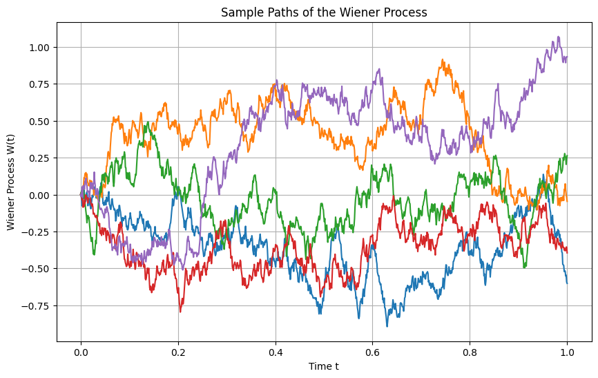
The Wiener Process

Simulation of the Wiener process (univariate)

import matplotlib.pyplot as plt
import numpy as np

# Set the parameters for the Wiener process
T = 1.0  # total time
n = 1000  # number of steps
dt = T / n  # time increment
t = np.linspace(0, T, n+1)  # time points

# Number of paths to simulate
num_paths = 5

# Set up the plot
plt.figure(figsize=(10, 6))

# Simulate multiple paths
for _ in range(num_paths):
    W = np.zeros(n+1)  # Initialize the Wiener process for each path
    for i in range(n):
        W[i+1] = W[i] + np.sqrt(dt) * np.random.randn()
    plt.plot(t, W, label=f'Path {_+1}')

# Customize the plot
plt.title('Sample Paths of the Wiener Process')
plt.xlabel('Time t')
plt.ylabel('Wiener Process W(t)')
plt.grid(True)

# Show the plot
plt.show()

Simulation using Gaussian processes

    import GPy
    import numpy as np
    import matplotlib.pyplot as plt

    # Time points at which to sample the Wiener process
    t = np.linspace(0, 1, 1000).reshape(-1, 1)

    # Define the Brownian motion kernel
    brownian_kernel = GPy.kern.Brownian(input_dim=1, variance=1.0)

    # Create a GP model with zero mean function
    mean_function = GPy.mappings.Constant(input_dim=1, output_dim=1, value=0)
    model = GPy.models.GPRegression(t, np.zeros_like(t), kernel=brownian_kernel, mean_function=mean_function)

    # Ensure correct model optimization
    model.optimize()

    # Sample paths from the GP model
    num_samples = 5
    samples = model.posterior_samples_f(t, size=num_samples)

    # Plot the sampled paths
    plt.figure(figsize=(10, 6))
    for i in range(num_samples):
        plt.plot(t, samples[:, :, i], label=f'Sample {i+1}')
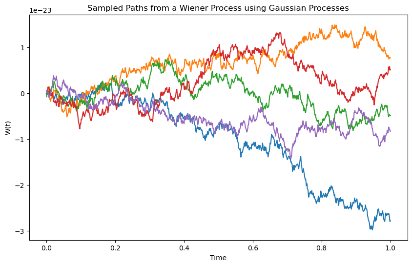
    plt.title('Sampled Paths from a Wiener Process using Gaussian Processes')
    plt.xlabel('Time')
    plt.ylabel('W(t)')
    plt.show()

Brownian motion with drift

Simulation using discrete paths

import matplotlib.pyplot as plt
import numpy as np

# Set the parameters for Brownian motion with drift and volatility
T = 1.0    # total time
n = 1000   # number of steps
dt = T / n  # time increment
t = np.linspace(0, T, n+1)  # time points

# Brownian motion parameters
mu = 5    # drift
sigma = 2.0  # volatility

# Number of paths to simulate
num_paths = 5

# Set up the plot
plt.figure(figsize=(10, 6))

# Simulate multiple paths
for _ in range(num_paths):
    X = np.zeros(n+1)  # Initialize the process for each path
    for i in range(n):
        X[i+1] = X[i] + mu * dt + sigma * np.sqrt(dt) * np.random.randn()
    plt.plot(t, X, label=f'Path {_+1}')

# Customize the plot
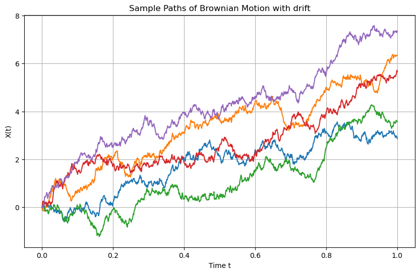
plt.title('Sample Paths of Brownian Motion with drift')
plt.xlabel('Time t')
plt.ylabel('X(t)')
plt.grid(True)

# Show the plot
plt.show()

Simulation using Gaussian Processes

import GPy
import numpy as np
import matplotlib.pyplot as plt

# Parameters for Brownian motion with drift
S0 = 0.0    # Initial value
mu = 0.5    # Drift coefficient
sigma = 0.3  # Volatility
T = 1.0    # Total time
n = 1000   # Number of steps
t = np.linspace(0, T, n+1).reshape(-1, 1)  # Time points

# Define the custom kernel for Brownian motion
class BrownianMotionKernel(GPy.kern.Kern):
    def __init__(self, input_dim, sigma=1.0, active_dims=None):
        super(BrownianMotionKernel, self).__init__(input_dim, active_dims, 'Brownian')
        self.sigma = GPy.core.Param('sigma', sigma)
        self.link_parameters(self.sigma)
    
    def K(self, X, X2=None):
        if X2 is None:
            X2 = X
        t1 = X
        t2 = X2.T
        # Covariance function of Brownian motion: sigma^2 * min(s, t)
        cov_matrix = self.sigma**2 * np.minimum(t1, t2)
        return cov_matrix
    
    def Kdiag(self, X):
        return self.sigma**2 * X[:, 0]
    
    # No-op for gradient update since we are not optimizing the kernel
    def update_gradients_full(self, dL_dK, X, X2=None):
        pass
    
    # No-op for kernel gradient since we are not optimizing the kernel
    def gradients_X(self, dL_dK, X, X2=None):
        return np.zeros(X.shape)

# Custom mean function to include drift
class BrownianMotionMean(GPy.core.Mapping):
    def __init__(self, input_dim, output_dim, S0=0.0, mu=0.0):
        super(BrownianMotionMean, self).__init__(input_dim, output_dim)
        self.S0 = S0  # Initial value
        self.mu = mu  # Drift coefficient
        
    def f(self, X):
        # Mean function: S0 + mu * t
        return self.S0 + self.mu * X
    
    def update_gradients(self, dL_df, X):
        pass

    def gradients_X(self, dL_df, X):
        return np.zeros(X.shape)

# Instantiate the Brownian motion kernel with parameters
bm_kernel = BrownianMotionKernel(input_dim=1, sigma=sigma)

# Instantiate the mean function with S0 and mu
mean_function = BrownianMotionMean(input_dim=1, output_dim=1, S0=S0, mu=mu)

# Provide the initial observation at t=0
t_data = np.array([[0.0]])
Y_data = np.array([[S0]])

# Create a GP model with the custom mean function and Brownian motion kernel
model = GPy.models.GPRegression(t_data, Y_data, kernel=bm_kernel, mean_function=mean_function)

# Set noise variance to a negligible value since we're simulating without observation noise
model.likelihood.variance.fix(1e-10)

# Sample paths from the GP model
num_samples = 5
samples = model.posterior_samples_f(t, size=num_samples)

# Plot the sampled paths
plt.figure(figsize=(10, 6))
for i in range(num_samples):
    plt.plot(t, samples[:, :, i], label=f'Path {i+1}')
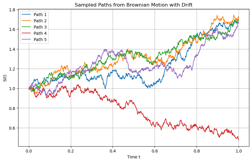
plt.title(f'Sampled Paths from Brownian Motion with Drift')
plt.xlabel('Time t')
plt.ylabel('S(t)')
plt.grid(True)
plt.legend()
plt.show()

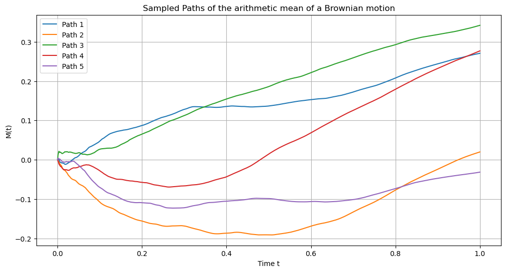
Arithmetic Average of the Brownian Motion

Simulation using discrete paths

import matplotlib.pyplot as plt
import numpy as np

# Set the parameters for Brownian motion with drift and volatility
T = 1.0    # total time
n = 1000   # number of steps
dt = T / n  # time increment
t = np.linspace(dt, T, n)  # time points starting from dt to avoid division by zero

# Brownian motion parameters
S0 = 0.0   # initial value of S_u
mu = 0.5   # drift coefficient
sigma = 0.3  # volatility

# Number of paths to simulate
num_paths = 5

# Initialize array to store M_t for each path
M_t_paths = np.zeros((n, num_paths))

# Set up the plot
plt.figure(figsize=(12, 6))

# Simulate multiple paths
for path in range(num_paths):
    # Initialize S_u for each path
    S = np.zeros(n + 1)  # n+1 because we include S0
    S[0] = S0
    # Simulate S_u using Euler-Maruyama method
    for i in range(n):
        dW = np.sqrt(dt) * np.random.randn()  # Brownian increment
        S[i + 1] = S[i] + mu * dt + sigma * dW
    # Compute cumulative sum to approximate the integral
    cumulative_S = np.cumsum(S[:-1]) * dt  # Exclude the last S[n+1]
    # Compute M_t at each time point
    M_t = cumulative_S / t
    M_t_paths[:, path] = M_t
    # Plot the path
    plt.plot(t, M_t, label=f'Path {path + 1}')

# Customize the plot
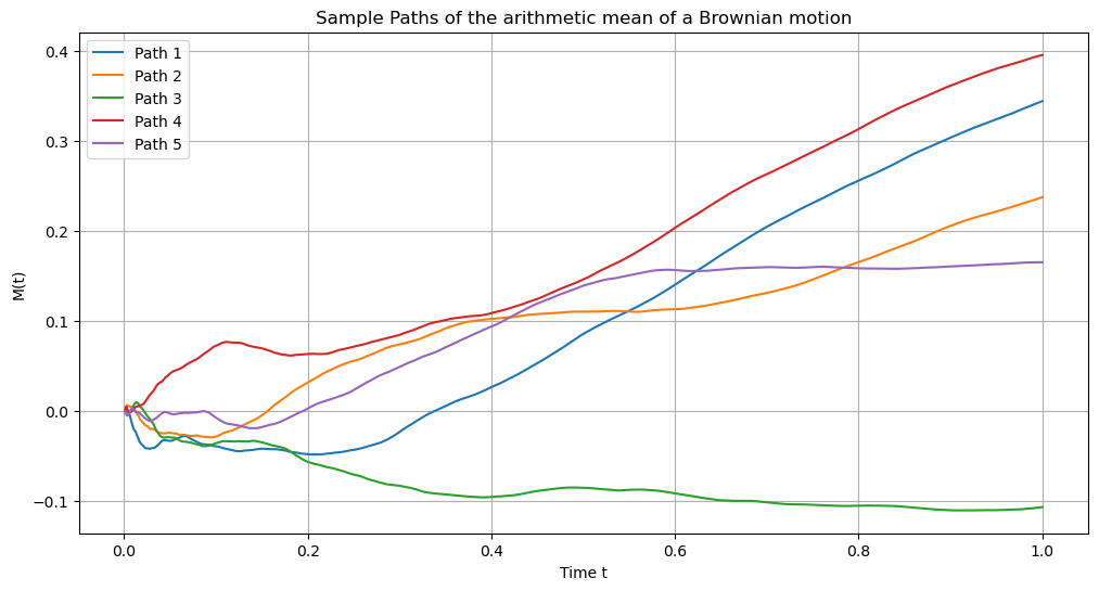
plt.title('Sample Paths of the arithmetic mean of a Brownian motion')
plt.xlabel('Time t')
plt.ylabel('M(t)')
plt.grid(True)
plt.legend()

# Show the plot
plt.show()

Simulation using Gaussian Processes

import GPy
import numpy as np
import matplotlib.pyplot as plt

# Parameters for Brownian motion with drift
S0 = 0.0    # Initial value
mu = 0.5    # Drift coefficient
sigma = 0.3  # Volatility
T = 1.0    # Total time
n = 1000   # Number of steps
t = np.linspace(1e-6, T, n+1).reshape(-1, 1)  # Time points, avoid t=0 to prevent division by zero

# Define the custom kernel based on the provided covariance function
class TimeAverageKernel(GPy.kern.Kern):
    def __init__(self, input_dim, sigma=1.0, active_dims=None):
        super(TimeAverageKernel, self).__init__(input_dim, active_dims, 'TimeAverage')
        self.sigma = GPy.core.Param('sigma', sigma)
        self.link_parameters(self.sigma)
        
    def K(self, X, X2=None):
        if X2 is None:
            X2 = X
        t1 = X[:, 0].reshape(-1, 1)  # Column vector
        t2 = X2[:, 0].reshape(1, -1)  # Row vector
        t_min = np.minimum(t1, t2)
        t_max = np.maximum(t1, t2)
        # Compute the covariance matrix using the given formula
        cov_matrix = self.sigma ** 2 * (t_min / 2) * (1 - t_min / (3 * t_max))
        return cov_matrix
        
    def Kdiag(self, X):
        t = X[:, 0]
        # Compute the diagonal elements of the covariance matrix
        cov_diag = self.sigma ** 2 * (t / 2) * (1 - t / (3 * t))
        # Simplify the expression
        cov_diag = self.sigma ** 2 * (t / 2) * (1 - 1 / 3)
        cov_diag = self.sigma ** 2 * (t / 2) * (2 / 3)
        cov_diag = self.sigma ** 2 * t * (1 / 3)
        return cov_diag
        
    def update_gradients_full(self, dL_dK, X, X2=None):
        pass
        
    def gradients_X(self, dL_dK, X, X2=None):
        return np.zeros(X.shape)

# Custom mean function to include drift
class TimeAverageMean(GPy.core.Mapping):
    def __init__(self, input_dim, output_dim, S0=0.0, mu=0.0):
        super(TimeAverageMean, self).__init__(input_dim, output_dim)
        self.S0 = S0  # Initial value
        self.mu = mu  # Drift coefficient
        
    def f(self, X):
        t = X[:, 0]
        mean = self.S0 + 0.5 * self.mu * t
        return mean.reshape(-1, 1)
        
    def update_gradients(self, dL_df, X):
        pass
    
    def gradients_X(self, dL_df, X):
        return np.zeros(X.shape)

# Instantiate the Time Average kernel with parameters
ta_kernel = TimeAverageKernel(input_dim=1, sigma=sigma)

# Instantiate the mean function with S0 and mu
mean_function = TimeAverageMean(input_dim=1, output_dim=1, S0=S0, mu=mu)

# Provide the initial observation at t=1e-6 (approaching zero)
t_data = np.array([[1e-6]])
Y_data = mean_function.f(t_data)  # Mean at t=1e-6

# Create a GP model with the custom mean function and Time Average kernel
model = GPy.models.GPRegression(t_data, Y_data, kernel=ta_kernel, mean_function=mean_function)

# Set noise variance to a negligible value since we're simulating without observation noise
model.likelihood.variance.fix(1e-10)

# Sample paths from the GP model
num_samples = 5
samples = model.posterior_samples_f(t, size=num_samples)

# Plot the sampled paths
plt.figure(figsize=(12, 6))
for i in range(num_samples):
    plt.plot(t, samples[:, :, i], label=f'Path {i+1}')
plt.title('Sampled Paths of the arithmetic mean of a Brownian motion')
plt.xlabel('Time t')
plt.ylabel('M(t)')
plt.grid(True)
plt.legend()
plt.show()

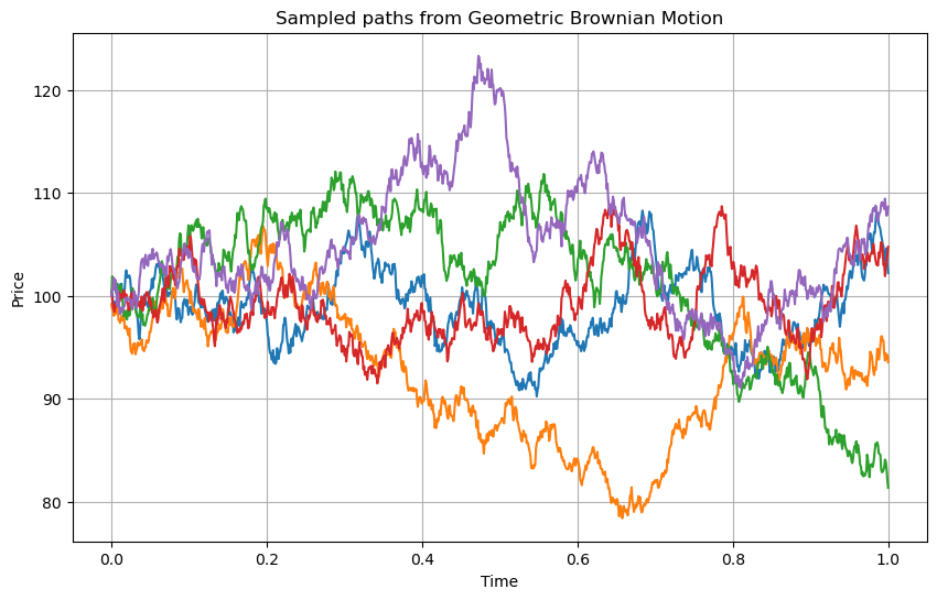
Geometric Brownian Motion

Simulation using discrete paths

import numpy as np
import matplotlib.pyplot as plt

def simulate_gbm(S0, mu, sigma, T, N, num_paths):
    dt = T / N
    t = np.linspace(0, T, N)
    paths = []
    for _ in range(num_paths):
        W = np.random.normal(0, np.sqrt(dt), N)
        W = np.cumsum(W)  # cumulative sum to represent Brownian motion
        S = S0 * np.exp((mu - 0.5 * sigma**2) * t + sigma * W)
        paths.append(S)
    return t, paths

# Parameters
S0 = 100  # Initial value of the asset
mu = 0.05  # Drift
sigma = 0.2  # Volatility
T = 1  # Time horizon (1 year)
N = 1000  # Number of time steps
num_paths = 5  # Number of paths to simulate

t, paths = simulate_gbm(S0, mu, sigma, T, N, num_paths)

# Plotting the simulated GBM paths
plt.figure(figsize=(10, 6))
for i, S in enumerate(paths):
    plt.plot(t, S, label=f'Path {i + 1}')
plt.xlabel('Time')
plt.ylabel('Price')
plt.title('Sampled paths from Geometric Brownian Motion')
plt.grid(True)
plt.show()

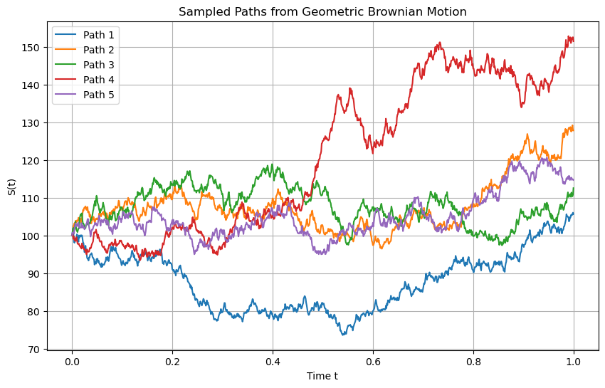
Simulation using Gaussian Processes

import GPy
import numpy as np
import matplotlib.pyplot as plt

# Parameters for Geometric Brownian Motion
S0 = 100  # Initial value of the asset
mu = 0.05  # Drift
sigma = 0.2  # Volatility
T = 1  # Time horizon (1 year)
n = 1000   # Number of steps
t = np.linspace(0, T, n+1).reshape(-1, 1)  # Time points

# Define the custom kernel for Brownian motion
class GBMKernel(GPy.kern.Kern):
    def __init__(self, input_dim, sigma=1.0, active_dims=None):
        super(GBMKernel, self).__init__(input_dim, active_dims, 'Brownian')
        self.sigma = GPy.core.Param('sigma', sigma)
        self.link_parameters(self.sigma)
    
    def K(self, X, X2=None):
        if X2 is None:
            X2 = X
        t1 = X
        t2 = X2.T
        # Covariance function of Brownian motion: sigma^2 * min(s, t)
        cov_matrix = self.sigma**2 * np.minimum(t1, t2)
        return cov_matrix
    
    def Kdiag(self, X):
        return self.sigma**2 * X[:, 0]
    
    # No-op for gradient update since we are not optimizing the kernel
    def update_gradients_full(self, dL_dK, X, X2=None):
        pass
    
    # No-op for kernel gradient since we are not optimizing the kernel
    def gradients_X(self, dL_dK, X, X2=None):
        return np.zeros(X.shape)

# Custom mean function to include drift
class GBMMean(GPy.core.Mapping):
    def __init__(self, input_dim, output_dim, S0=0.0, mu=0.0):
        super(GBMMean, self).__init__(input_dim, output_dim)
        self.S0 = S0  # Initial value
        self.mu = mu  # Drift coefficient
        
    def f(self, X):
        # Mean function: S0 + mu * t
        return self.S0 + self.mu * X
    
    def update_gradients(self, dL_df, X):
        pass

    def gradients_X(self, dL_df, X):
        return np.zeros(X.shape)

# Instantiate the Brownian motion kernel with parameters
bm_kernel = GBMKernel(input_dim=1, sigma=sigma)

# Instantiate the mean function with S0 and mu
mean_function = GBMMean(input_dim=1, output_dim=1, S0=np.log(S0), mu=mu)

# Provide the initial observation at t=0
t_data = np.array([[0.0]])
Y_data = np.array([[np.log(S0)]])

# Create a GP model with the custom mean function and Brownian motion kernel
model = GPy.models.GPRegression(t_data, Y_data, kernel=bm_kernel, mean_function=mean_function)

# Set noise variance to a negligible value since we're simulating without observation noise
model.likelihood.variance.fix(1e-10)

# Sample paths from the GP model
num_samples = 5
samples = model.posterior_samples_f(t, size=num_samples)

# Transform samples to original GBM scale
gbm_samples = np.exp(samples)

# Plot the sampled paths
plt.figure(figsize=(10, 6))
for i in range(num_samples):
    plt.plot(t, gbm_samples[:, :, i], label=f'Path {i+1}')
plt.title(f'Sampled Paths from Geometric Brownian Motion')
plt.xlabel('Time t')
plt.ylabel('S(t)')
plt.grid(True)
plt.legend()
plt.show()

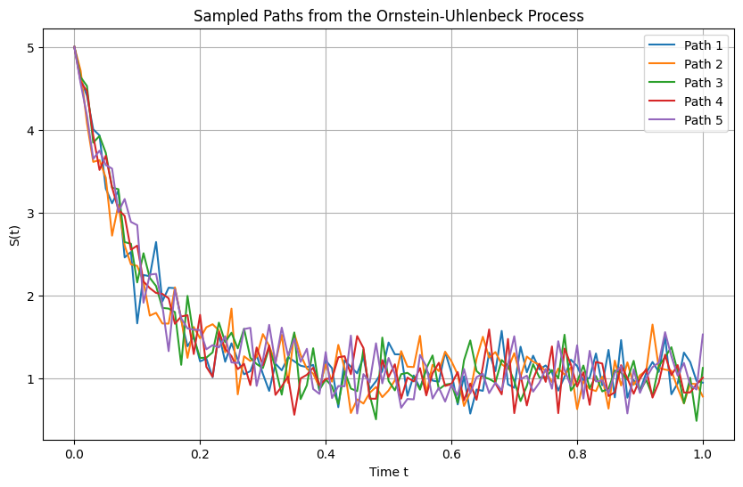
Orstein - Uhlenbeck process

Simulation using discrete paths

import numpy as np
import matplotlib.pyplot as plt

# Parameters for the Ornstein-Uhlenbeck process
S0 = 5.0    # Initial value
mu = 1.0    # Long-term mean
theta = 10  # Rate of mean reversion
sigma = 1 # Volatility
T = 1.0    # Total time
n = 100   # Number of steps
dt = T / n  # Time step size
t = np.linspace(0, T, n+1)  # Time points

# Number of paths to simulate
num_paths = 5

# Set up the plot
plt.figure(figsize=(10, 6))

# Simulate multiple paths
for _ in range(num_paths):
    S = np.zeros(n+1)  # Initialize the process
    S[0] = S0  # Set initial value

    for i in range(1, n+1):
        # Compute the mean and variance for the next step
        mean = S0 * np.exp(-theta * t[i]) + mu * (1 - np.exp(-theta * t[i]))
        variance = (sigma**2 / (2 * theta)) * (1 - np.exp(-2 * theta * t[i]))
        
        # Sample from the normal distribution with the computed mean and variance
        S[i] = np.random.normal(mean, np.sqrt(variance))

    # Plot the Ornstein-Uhlenbeck path
    plt.plot(t, S, label=f'Path {_+1}')

# Customize the plot
plt.title('Sampled Paths from the Ornstein-Uhlenbeck Process')
plt.xlabel('Time t')
plt.ylabel('S(t)')
plt.grid(True)
plt.legend()
plt.show()

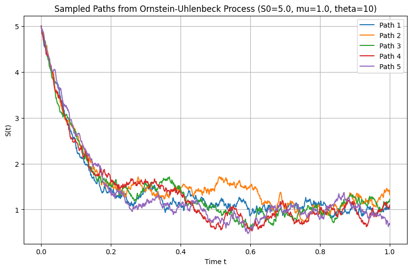
Simulation using Gaussian Processes

import GPy
import numpy as np
import matplotlib.pyplot as plt

# Parameters for the Ornstein-Uhlenbeck process
S0 = 5.0    # Initial value
mu = 1.0    # Long-term mean
theta = 10  # Rate of mean reversion
sigma = 1 # Volatility
T = 1.0    # Total time
n = 1000   # Number of steps
t = np.linspace(0, T, n+1).reshape(-1, 1)  # Time points

# Define the custom kernel for the Ornstein-Uhlenbeck process
class OrnsteinUhlenbeckKernel(GPy.kern.Kern):
    def __init__(self, input_dim, theta=1.0, sigma=1.0, active_dims=None):
        super(OrnsteinUhlenbeckKernel, self).__init__(input_dim, active_dims, 'OU')
        self.theta = GPy.core.Param('theta', theta)
        self.sigma = GPy.core.Param('sigma', sigma)
        self.link_parameters(self.theta, self.sigma)
    
    def K(self, X, X2=None):
        if X2 is None:
            X2 = X
        t1 = X
        t2 = X2.T
        min_t = np.minimum(t1, t2)
        # Covariance function of the Ornstein-Uhlenbeck process
        cov_matrix = (self.sigma**2 / (2 * self.theta)) * np.exp(-self.theta * np.abs(t1 - t2)) * (1 - np.exp(-2 * self.theta * min_t))
        return cov_matrix
    
    def Kdiag(self, X):
        return (self.sigma**2 / (2 * self.theta)) * (1 - np.exp(-2 * self.theta * X[:, 0]))
    
    # No-op for gradient update since we are not optimizing the kernel
    def update_gradients_full(self, dL_dK, X, X2=None):
        pass
    
    # No-op for kernel gradient since we are not optimizing the kernel
    def gradients_X(self, dL_dK, X, X2=None):
        return np.zeros(X.shape)

# Custom mean function to include mean-reverting drift toward mu
class OUProcessMean(GPy.core.Mapping):
    def __init__(self, input_dim, output_dim, S0=0.0, mu=0.0, theta=1.0):
        super(OUProcessMean, self).__init__(input_dim, output_dim)
        self.S0 = S0  # Initial value
        self.mu = mu  # Long-term mean
        self.theta = theta  # Rate of mean reversion
        
    def f(self, X):
        # Mean function: S_0 * exp(-theta * t) + mu * (1 - exp(-theta * t))
        return self.S0 * np.exp(-self.theta * X) + self.mu * (1 - np.exp(-self.theta * X))
        
    def update_gradients(self, dL_df, X):
        pass
    
    def gradients_X(self, dL_df, X):
        return np.zeros(X.shape)

# Instantiate the OU kernel with parameters
ou_kernel = OrnsteinUhlenbeckKernel(input_dim=1, theta=theta, sigma=sigma)

# Instantiate the mean function with non-zero initial value S0 and long-term mean mu
mean_function = OUProcessMean(input_dim=1, output_dim=1, S0=S0, mu=mu, theta=theta)

# Provide the initial observation at t=0
t_data = np.array([[0.0]])
Y_data = np.array([[S0]])

# Create a GP model with the custom mean function and OU kernel
model = GPy.models.GPRegression(t_data, Y_data, kernel=ou_kernel, mean_function=mean_function)

# Set noise variance to a negligible value since we're simulating without observation noise
model.likelihood.variance.fix(1e-10)

# Sample paths from the GP model
num_samples = 5
samples = model.posterior_samples_f(t, size=num_samples)

# Plot the sampled paths
plt.figure(figsize=(10, 6))
for i in range(num_samples):
    plt.plot(t, samples[:, :, i], label=f'Path {i+1}')
plt.title(f'Sampled Paths from Ornstein-Uhlenbeck Process (S0={S0}, mu={mu}, theta={theta})')
plt.xlabel('Time t')
plt.ylabel('S(t)')
plt.grid(True)
plt.legend()
plt.show()

Brownian bridge

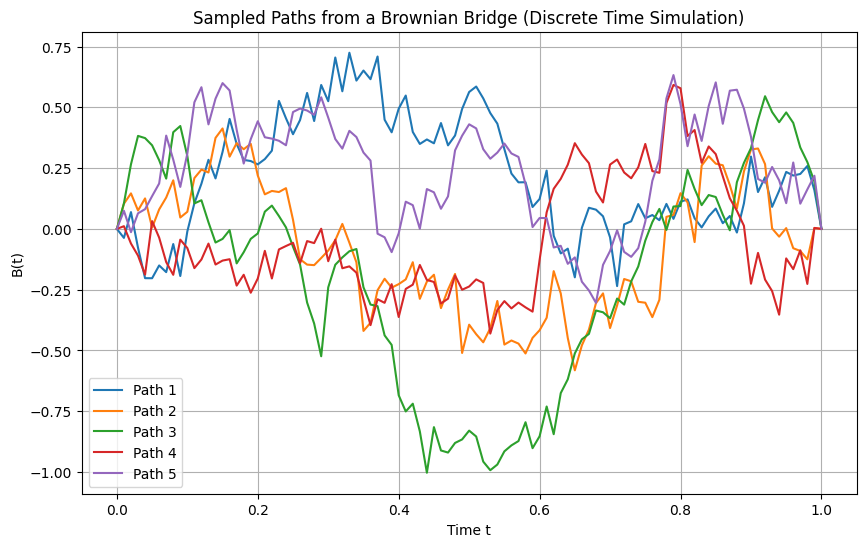
Simulation using discrete paths

import numpy as np
import matplotlib.pyplot as plt

# Parameters for the Brownian bridge
T = 1.0    # Total time
n = 100   # Number of steps
dt = T / n  # Time step size
t = np.linspace(0, T, n+1)  # Time points

# Number of paths to simulate
num_paths = 5

# Set up the plot
plt.figure(figsize=(10, 6))

# Simulate multiple paths
for _ in range(num_paths):
    W = np.zeros(n+1)  # Initialize the Wiener process
    for i in range(1, n+1):
        W[i] = W[i-1] + np.sqrt(dt) * np.random.randn()  # Standard Wiener process

    # Adjust Wiener process to form a Brownian bridge
    B = W - (t / T) * W[-1]  # Brownian bridge: W(t) - (t/T) * W(T)

    # Plot the Brownian bridge path
    plt.plot(t, B, label=f'Path {_+1}')

# Customize the plot
plt.title('Sampled Paths from a Brownian Bridge (Discrete Time Simulation)')
plt.xlabel('Time t')
plt.ylabel('B(t)')
plt.grid(True)
plt.legend()
plt.show()

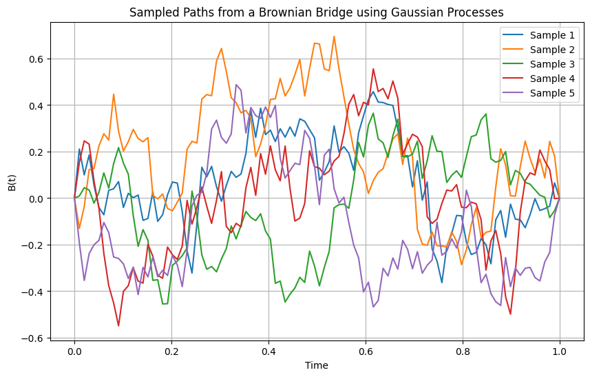
Simulation using Gaussian processes

import GPy
import numpy as np
import matplotlib.pyplot as plt

# Time points at which to sample the Brownian bridge
T = 1.0
t = np.linspace(0, T, 100).reshape(-1, 1)

# Define a custom kernel for the Brownian bridge
class BrownianBridgeKernel(GPy.kern.Kern):
    def __init__(self, input_dim, variance=1.0, active_dims=None):
        super(BrownianBridgeKernel, self).__init__(input_dim, active_dims, 'brownian_bridge')
        self.variance = GPy.core.Param('variance', variance)
        self.link_parameter(self.variance)
    
    def K(self, X, X2=None):
        if X2 is None:
            X2 = X
        t1 = X
        t2 = X2.T
        T = np.max(X)
        # Brownian bridge kernel: min(t1, t2) - (t1 * t2) / T
        cov_matrix = np.minimum(t1, t2) - (t1 * t2) / T
        return self.variance * cov_matrix
    
    def Kdiag(self, X):
        return self.variance * (X[:, 0] - (X[:, 0]**2) / T)
    
    # No-op for gradient update since we are not optimizing the kernel
    def update_gradients_full(self, dL_dK, X, X2=None):
        pass
    
    # No-op for kernel gradient since we are not optimizing the kernel
    def gradients_X(self, dL_dK, X, X2=None):
        return np.zeros(X.shape)

# Instantiate the Brownian bridge kernel with variance 1
brownian_bridge_kernel = BrownianBridgeKernel(input_dim=1, variance=1.0)

# Create a GP model with zero mean function
mean_function = GPy.mappings.Constant(input_dim=1, output_dim=1, value=0)
model = GPy.models.GPRegression(t, np.zeros_like(t), kernel=brownian_bridge_kernel, mean_function=mean_function)

# Sample paths from the GP model without optimizing (since Brownian bridge doesn't require fitting)
num_samples = 5
samples = model.posterior_samples_f(t, size=num_samples)

# Plot the sampled paths
plt.figure(figsize=(10, 6))
for i in range(num_samples):
    plt.plot(t, samples[:, :, i], label=f'Sample {i+1}')
plt.title('Sampled Paths from a Brownian Bridge using Gaussian Processes')
plt.xlabel('Time')
plt.ylabel('B(t)')
plt.grid(True)
plt.legend()
plt.show()

Jump processes

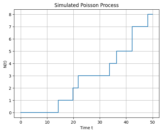
Homogeneous Poisson process simulation

import numpy as np
import matplotlib.pyplot as plt

# Parameters
lambda_rate = 0.2   # The rate parameter λ of the Poisson process
T = 50             # Total time
delta_t = 0.01      # Time-step Δt
num_steps = int(T / delta_t)  # Number of time steps

# Time grid
t = np.linspace(0, T, num_steps + 1)

# Initialize N_t
N_t = np.zeros(num_steps + 1, dtype=int)

# Simulate the Poisson process
for i in range(1, num_steps + 1):
    # Generate a random number between 0 and 1
    u = np.random.rand()
    # If u < λΔt, increment N_t
    if u < lambda_rate * delta_t:
        N_t[i] = N_t[i - 1] + 1
    else:
        N_t[i] = N_t[i - 1]

# Plot the Poisson process
plt.step(t, N_t, where='post')
plt.xlabel('Time t')
plt.ylabel('N(t)')
plt.title('Simulated Poisson Process')
plt.grid(True)
plt.show()

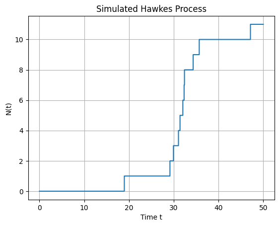
Hawkes process

import numpy as np
import matplotlib.pyplot as plt

# Parameters
mu = 0.2       # Baseline intensity (μ)
alpha = 0.5   # Excitation parameter (α)
beta = 1     # Decay rate (β)
T = 50         # Total time to simulate
delta_t = 0.01 # Time-step Δt

# Time grid
time_grid = np.arange(0, T + delta_t, delta_t)
num_steps = len(time_grid)

# Initialize N_t and event times
N_t = np.zeros(num_steps, dtype=int)
event_times = []

# Simulate the Hawkes process
for i in range(1, num_steps):
    t_i = time_grid[i]
    
    # Compute lambda_t
    lambda_t = mu
    if event_times:
        tau_array = np.array(event_times)
        lambda_t += np.sum(alpha * np.exp(-beta * (t_i - tau_array)))
    
    # Calculate the event probability
    p = lambda_t * delta_t
    if p > 1.0:
        p = 1.0  # Ensure probability does not exceed 1
    
    # Simulate event occurrence
    u = np.random.rand()
    if u < p:
        N_t[i] = N_t[i - 1] + 1
        event_times.append(t_i)
    else:
        N_t[i] = N_t[i - 1]

# Plot the counting process
#plt.figure(figsize=(12, 6))
plt.step(time_grid, N_t, where='post')
plt.xlabel('Time t')
plt.ylabel('N(t)')
plt.title('Simulated Hawkes Process')
plt.grid(True)
plt.show()

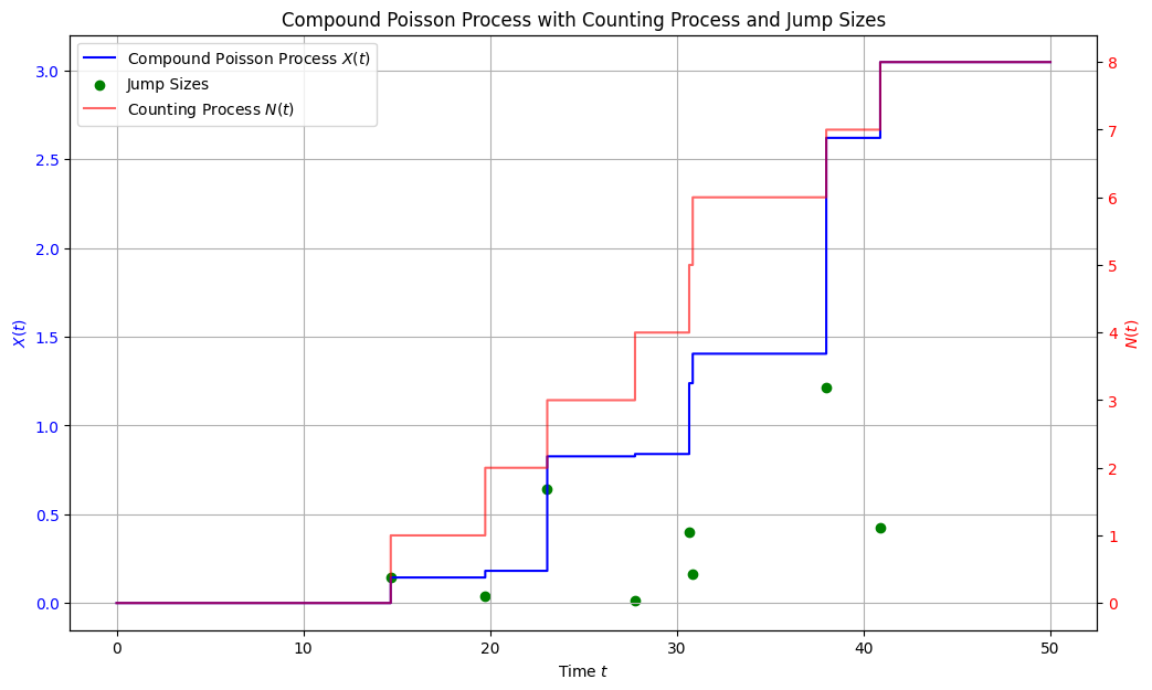
Compound Poisson process

import numpy as np
import matplotlib.pyplot as plt

# Parameters
lambda_rate = 0.2   # Rate parameter λ of the Poisson process
T = 50              # Total simulation time
delta_t = 0.01      # Time-step Δt
num_steps = int(T / delta_t)
time_grid = np.linspace(0, T, num_steps + 1)

# Jump size distribution parameters
eta = 2.5  # Rate parameter of the exponential distribution for jump sizes

# Initialize arrays
N_t = np.zeros(num_steps + 1, dtype=int)  # Counting process N(t)
X_t = np.zeros(num_steps + 1)             # Compound Poisson process X(t)
event_times = []                          # Times when events occur
jump_sizes = []                           # Sizes of the jumps

# Simulate the compound Poisson process
for i in range(1, num_steps + 1):
    t = time_grid[i]
    # Probability of an event in [t_i, t_i + delta_t)
    p = lambda_rate * delta_t
    # Ensure probability does not exceed 1
    p = min(p, 1.0)
    # Determine if an event occurs
    if np.random.rand() < p:
        N_t[i] = N_t[i - 1] + 1
        # Sample a jump size Y_i from an exponential distribution
        Y_i = np.random.exponential(scale=1/eta)
        jump_sizes.append(Y_i)
        event_times.append(t)
        X_t[i] = X_t[i - 1] + Y_i
    else:
        N_t[i] = N_t[i - 1]
        X_t[i] = X_t[i - 1]

# Plot all three visualizations in one figure
fig, ax1 = plt.subplots(figsize=(12, 7))

# Plot the compound Poisson process X(t)
ax1.step(time_grid, X_t, where='post', label='Compound Poisson Process $X(t)$', color='blue')
ax1.set_xlabel('Time $t$')
ax1.set_ylabel('$X(t)$', color='blue')
ax1.tick_params(axis='y', labelcolor='blue')
ax1.grid(True)

# Plot jump sizes as scatter points on X(t)
event_indices = [np.searchsorted(time_grid, t) for t in event_times]
event_values = [X_t[idx] for idx in event_indices]
ax1.scatter(event_times, jump_sizes, color='green', marker='o', label='Jump Sizes')

# Create a secondary y-axis for the counting process N(t)
ax2 = ax1.twinx()
ax2.step(time_grid, N_t, where='post', label='Counting Process $N(t)$', color='red', alpha=0.6)
ax2.set_ylabel('$N(t)$', color='red')
ax2.tick_params(axis='y', labelcolor='red')

# Combine legends from both axes
lines1, labels1 = ax1.get_legend_handles_labels()
lines2, labels2 = ax2.get_legend_handles_labels()
ax1.legend(lines1 + lines2, labels1 + labels2, loc='upper left')

plt.title('Compound Poisson Process with Counting Process and Jump Sizes')
plt.show()

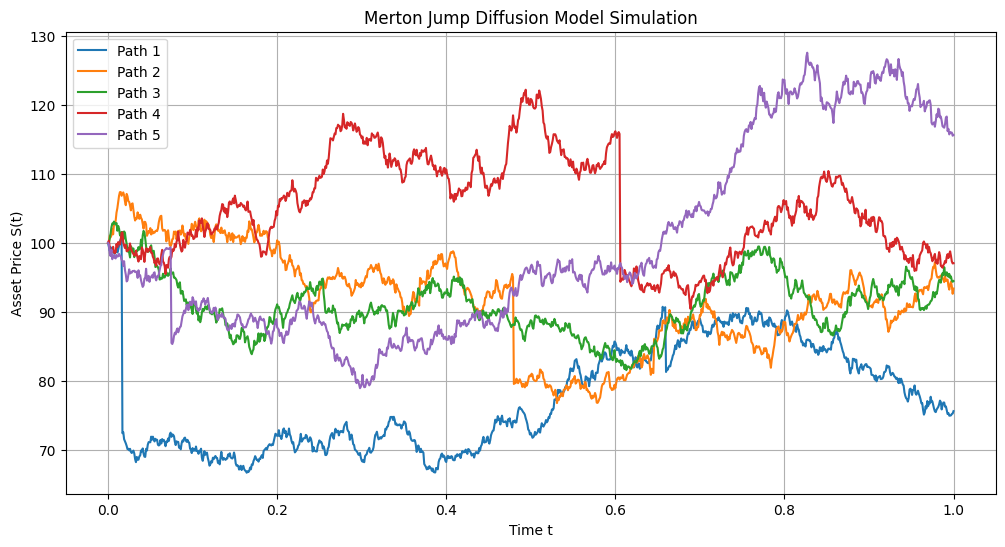
Jump diffusion processes

import numpy as np
import matplotlib.pyplot as plt

def simulate_merton_jump_diffusion(S0, mu, sigma, lamb, mu_j, sigma_j, T, N, M):
    """
    Simulate the Merton jump diffusion model.

    Parameters:
    - S0: Initial asset price.
    - mu: Expected return (drift rate).
    - sigma: Volatility of the continuous component.
    - lamb: Jump intensity (average number of jumps per unit time).
    - mu_j: Mean of the jump size distribution (of ln(J)).
    - sigma_j: Standard deviation of the jump size distribution (of ln(J)).
    - T: Total time horizon.
    - N: Number of time steps.
    - M: Number of simulation paths.

    Returns:
    - t: Array of time points.
    - S: Matrix of simulated asset prices (M paths x N+1 time points).
    """
    dt = T / N  # Time step size
    t = np.linspace(0, T, N + 1)  # Time grid

    # Precompute constants
    drift = (mu - 0.5 * sigma**2) * dt
    diffusion = sigma * np.sqrt(dt)

    # Initialize asset price paths
    S = np.zeros((M, N + 1))
    S[:, 0] = S0

    for m in range(M):
        # Initialize variables for each path
        S_m = np.zeros(N + 1)
        S_m[0] = S0

        # Generate random numbers for Brownian motion
        Z = np.random.normal(size=N)

        # Generate random numbers for jumps
        # Poisson random numbers for number of jumps in each time step
        Nt = np.random.poisson(lamb * dt, size=N)
        # Total number of jumps
        num_jumps = np.sum(Nt)
        # Generate jump sizes only where jumps occur
        if num_jumps > 0:
            jump_sizes = np.random.normal(loc=mu_j, scale=sigma_j, size=num_jumps)
        else:
            jump_sizes = np.array([])

        # Index to keep track of jump sizes
        jump_index = 0

        for i in range(1, N + 1):
            # Continuous part
            S_m[i] = S_m[i - 1] * np.exp(drift + diffusion * Z[i - 1])

            # Jump part
            if Nt[i - 1] > 0:
                # Apply jumps
                total_jump = np.sum(jump_sizes[jump_index:jump_index + Nt[i - 1]])
                S_m[i] *= np.exp(total_jump)
                jump_index += Nt[i - 1]

        S[m, :] = S_m

    return t, S

# Parameters
S0 = 100        # Initial asset price
mu = 0.1        # Expected return
sigma = 0.2     # Volatility
lamb = 1     # Jump intensity λ
k = -0.1     # Mean of ln(J) (jump sizes)
delta = 0.1   # Std dev of ln(J)
T = 1.0         # Total time (e.g., 1 year)
N = 1000        # Number of time steps
M = 5           # Number of simulation paths

# Simulate the Merton jump diffusion model
t, S = simulate_merton_jump_diffusion(S0, mu, sigma, lamb, k, delta, T, N, M)

# Plot the simulated asset price paths
plt.figure(figsize=(12, 6))
for m in range(M):
    plt.plot(t, S[m, :], label=f'Path {m + 1}')
plt.xlabel('Time t')
plt.ylabel('Asset Price S(t)')
plt.title('Merton Jump Diffusion Model Simulation')
plt.legend()
plt.grid(True)
plt.show()